The aim of this session is to complete the analysis of the RNA-seq data using the limma and edgeR packages. With the results of the analysis, we want to be able to produce publication quality figures and write out the results to a file for sharing or publication.
Learning Objectives
fit a linear model to the data
construct design and contrast matrices for the linear model
model the mean-variance relationship of the data using the voom() function
perform statistical testing to identify differentially expressed genes
visualise the results using an MA plot
write out the results to a file
# load required packageslibrary(tidyverse)
── Attaching core tidyverse packages ──────────────────────── tidyverse 2.0.0 ──
✔ dplyr     1.1.4     ✔ readr     2.1.5
✔ forcats   1.0.0     ✔ stringr   1.5.1
✔ ggplot2   3.5.1     ✔ tibble    3.2.1
✔ lubridate 1.9.3     ✔ tidyr     1.3.1
✔ purrr     1.0.2
── Conflicts ────────────────────────────────────────── tidyverse_conflicts() ──
✖ dplyr::filter() masks stats::filter()
✖ dplyr::lag()    masks stats::lag()
ℹ Use the conflicted package (<http://conflicted.r-lib.org/>) to force all conflicts to become errors
Rows: 27179 Columns: 3
── Column specification ────────────────────────────────────────────────────────
Delimiter: "\t"
chr (2): SYMBOL, TXCHROM
dbl (1): ENTREZID

ℹ Use `spec()` to retrieve the full column specification for this data.
ℹ Specify the column types or set `show_col_types = FALSE` to quiet this message.
# filter lowly expressed geneskeep <-filterByExpr(dge)dge <- dge[keep, ]# normalise the data for library size and RNA compositiondge <-calcNormFactors(dge, method ="TMM")
6.1 Linear modelling
To identify differentially expressed genes from our normalised gene expression data, we will use the limma package to fit linear models to the genes. A linear model is a broad class of statistical models that fit the value of an response (or dependent) variable as a linear function of one or more explanatory (or independent) variables (also called covariates).
The general form of a linear model looks like this:
This equation is saying that a response variable of interest \(Y\) is equal to a constant (\(\beta_{0}\)) plus the sum of the covariates (\(X_{i}\)) each multiplied by a constant coefficient (\(\beta_{i}\)) and some error term (\(\epsilon\)). The error term is the difference between the observed value and the predicted value of the model and is assumed to have a normal distribution with mean 0 and some variance.
Our experiment is quite simple, since there is only a single covariate, the cell type. The true benefit of using linear models is in its ability to accommodate more complex designs including multiple covariates.
To fit the linear models in the limma-voom framework we need two objects in addition to our data:
A design matrix, representing the covariates.
A contrast matrix, representing the specific comparison we wish to make.
6.1.1 Design matrix
The first step to fitting a linear model is to specify a design matrix. The design matrix specifies the values of the covariates for each sample, and is represented as a matrix due to the mathematical convenience.
To generate a design matrix. We use the function model.matrix(), with the expression ~0 + group. This returns a matrix representing the design where there is no intercept term and group is the only covariate. If we omit the 0 then there would be an intercept in the model, and if we included more covariates then more columns would be generated.
design <-model.matrix(~0+ group, data = dge$samples)design
There are 9 rows, one for each sample. Along the columns are the names of the groups. The values in the cells denote membership of the particular sample for a particular group, as our groups in this case are mutually exclusive, each row contains only a single 1 to denote membership in a single group.
6.1.2 Contrasts
Contrast matrices are companions to design matrices. They are used to specify the comparison of interest. In our case, we have three experimental groups: Basal, LP and ML. So if we are to perform differential expression analysis, we are most likely interested in the differences between only two of the groups at a time. Contrast matrices let use specify which comparison we’d like to make, and are also represented as a matrix just like the design.
A contrast matrix can be made using the makeContrasts() function. Within this function, we specify the name of each specific contrast and the formula for that contrast. For example, the BasalvsLP contrasts compares the difference between the Basal and LP groups. Note that the name of the phenotype groups must be written exactly as they are in the column names of our design matrix (see above).
In addition to the individual contrasts, the function must know about the design of the model. This is passed through the levels argument, which either accepts a matrix with the column names corresponding to levels of your experimental groups, or the levels themselves as a character vector. Here we first simplify the column names of our design matrix to make it easier to read. Then we create the contrast matrix using the makeContrasts() function.
There are two things to note about a design matrix. First, the sum of the numbers in each row is equal to 0. Second, the way that you set up the equation in the matrix will determine the interpretation of the log-fold-change calculated later, as well as the meaning of up-regulated and down-regulated genes. For example, the contrast Basal - LP will give a positive log-fold-change for genes that are up-regulated in the Basal group compared to the LP group. If we had set up the contrast as LP - Basal, then the opposite would be true, and we would get a negative log-fold-change for genes that are up-regulated in the Basal group compared to the LP group.
6.1.3 Variance modelling with voom
We are now ready to fit our linear models. Limma fits linear models to the data with the assumption that the underlying data is normally distributed. Count data is generally not normally distributed, but log transforming count data gives it a roughly normal distribution sufficient for linear models to work well. To do this, limma transforms the raw count data to log-cpm using library sizes and the normalisation factors we calculated previously.
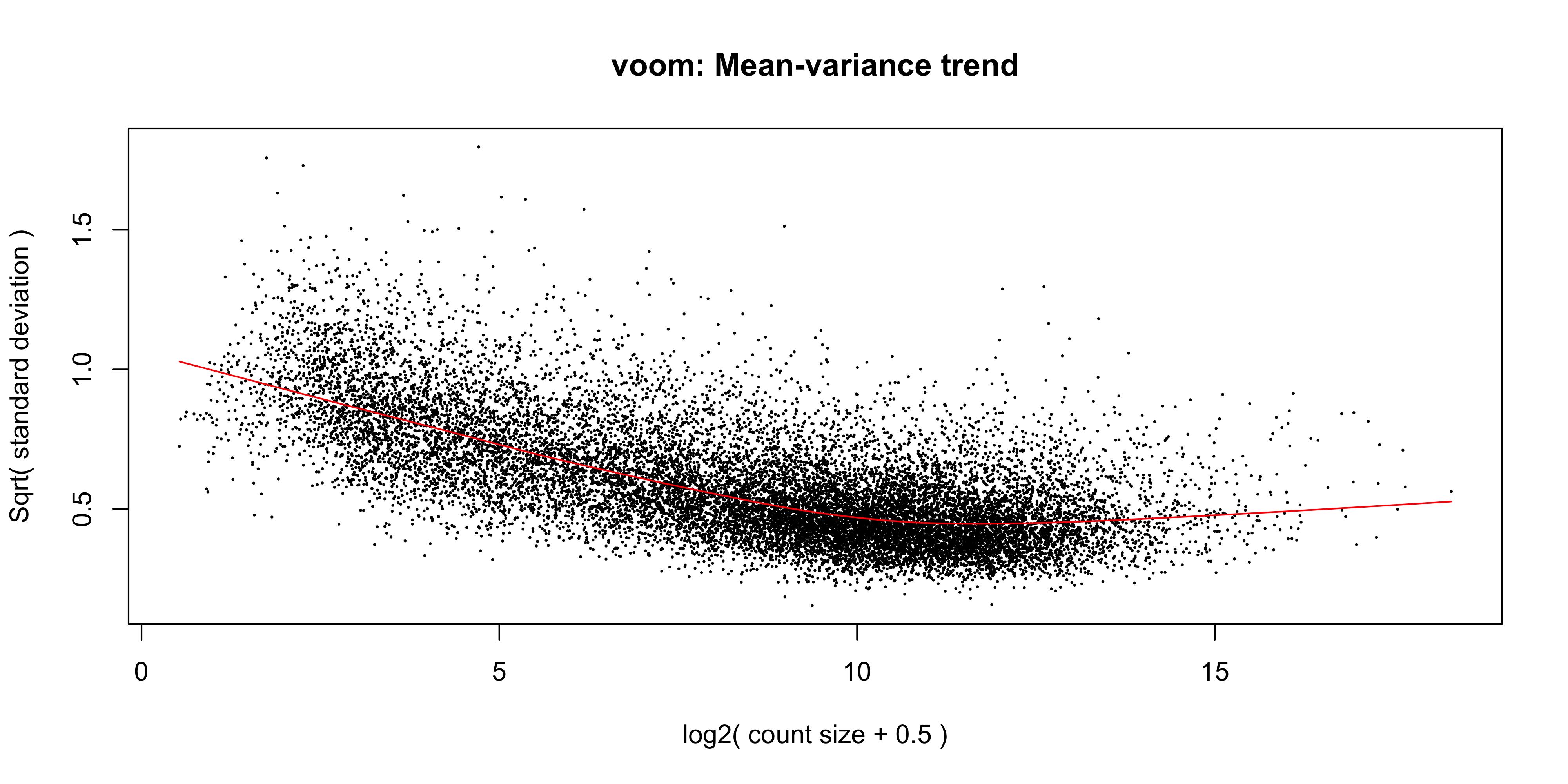
In addition to the normalisation steps, the limma-voom pipeline uses the voom() function to generate weights for the individual genes based on a modelled mean-variance relationship. This modelling allows use to get more information out of small sample sizes as the weights prevent our model from being more heavily influenced by more variable data points. The weights will then allow the linear model to be less influenced by genes with high variability, which is important for small sample sizes. The voom function also generates a mean-variance plot, which is useful for visualising the data.
The voom() function takes as arguments, our DGEList object and our design matrix. It also optionally outputs a plot of the mean-variance relationship of our data, called the ‘voom-plot’.
v <-voom(dge, design, plot =TRUE)
The output of voom() (our variable v) is an EList object which contains the following elements:
genes - a data frame of gene annotation data.
targets - data frame of sample data.
E - numeric matrix of normalised log-cpm values.
weights - numeric matrix of precision weights.
design - the design matrix.
The MA plot shows the mean-variance relationship of the data. The x-axis is the average log2 expression of each gene, and the y-axis is the log2 standard deviation of each gene. The idea is that the variance of a gene can be estimated as a function of its main expression, and that this estimate is more accurate than the direct calculation of the variance.
6.1.4 Fitting the linear model
We are now ready to fit our linear model with lmFit(), which calculates coefficients we defined in our design matrix design. The resulting object, vfit is a MArrayLM object. It contains a information about our genes (the same data frame as genes from our EList object v above), the design matrix and a number of statistical outputs. Of most interest to us is the coefficients, stored in an element called coefficients. The first rows of this matrix is shown below. Each gene is row and is labelled using the EntrezID. Each column gives coefficients for each of our phenotype groups. These coefficients are weighted averages of the log-cpm of each gene in each group.
We can then use contrasts.fit() to calculate coefficients for each contrast (or ‘comparison’) we specified in our contr_matrix. The output is also an object of the class MArrayLM (also known as an MArrayLM object). When we inspect the coefficients element now, we can see that each column is a contrast that we specified in our contrast matrix.
With these values we essentially want to know whether or not the difference in values is significantly different from 0. If the difference is not significantly different from 0, then we have failed to establish a difference in the expression of a particularly gene between two groups. If the difference is significantly greater than 0, then we have up-regulation in the first group of the contrast, and if the difference is significantly less than 0, then we have down-regulation in the first group of the contrast.
6.2 Statistical testing
To actually test if the values are significantly different from 0, we use the eBayes() function to compute moderated t-statistics, moderated F-statistics and log-odds of differential expression for each gene, given a fitted linear model. ‘Moderated’ refers to empirical Bayes moderation, which borrows information across genes to obtain more accurate measures of variability for each gene. This also increases our power to detect differentially expressed genes.
efit <-eBayes(vfit)
We can now look at the number of differentially expressed genes using the decideTests() function. The output of this function is a matrix where each column is a contrast (comparison of interest) and each row is a gene. The numbers 1, -1 and 0 mean up-regulated, down-regulated or not significantly differentially expressed, respectively.
Note that decideTests() also accounts for multiple testing. The default method is Benjamini and Hochberg1 but several others are also available.
To obtain the total number of differentially expressed genes for each comparison, we can add the function summary():
summary(dt)
       BasalvsLP BasalvsML LPvsML
Down        4501      4850   2701
NotSig      7306      6996  11821
Up          4817      4778   2102
The function topTable() can be used to obtain more information on the differentially expressed genes for each contrast. topTable() takes as arguments the MArrayLM object output by eBayes() (efit), the contrast name of interest and the number of top differentially expressed genes to output. Note that the contrast name must be given in quotes and must be exactly as written in the contrast matrix contr_matrix.
It outputs a data frame with the following information:
Gene details - gene information, from the gene element of the MArrayLM object (efit).
logFC - the log2 fold change of the contrast.
AveExpr - the average log2 expression of that gene.
t - moderated t-statistic.
P.Value - p value.
adj.P.Val - adjusted p value.
B - log-odds that the gene is differentially expressed.
top <-topTable(efit, coef ="BasalvsLP", n =Inf)head(top)
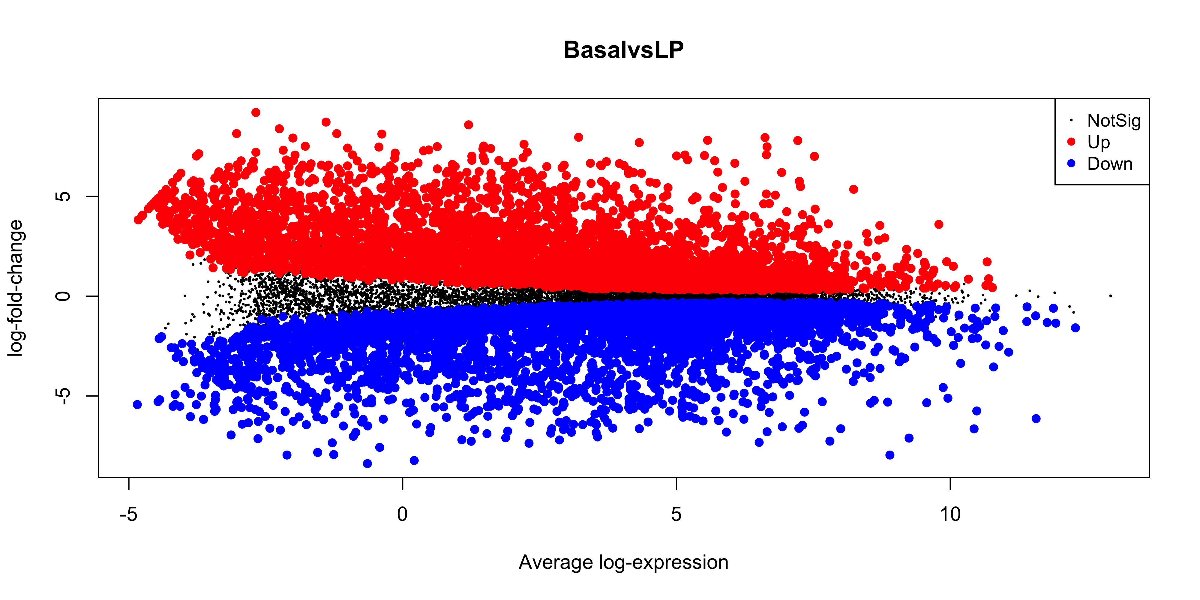
The MA plot is a plot of log-fold-change (M-values) against log-expression averages (A-values), this is a common plot in RNA sequencing analysis to visualise the result of differential expression tests. It can be created using the plotMA() from the limma package. Creating this plot requires 3 pieces of information:
object = efit: The the fitted object containing the log-fold-change and log-expression averages
coef = 1: The column number of the contrast to plot since there are 3 different contrasts fitted within the object.
status = dt[, 1]: A vector of numerics denoting whether a gene is up-regulated or down-regulated.
plotMA(efit, coef =1, status = dt[, "BasalvsLP"])
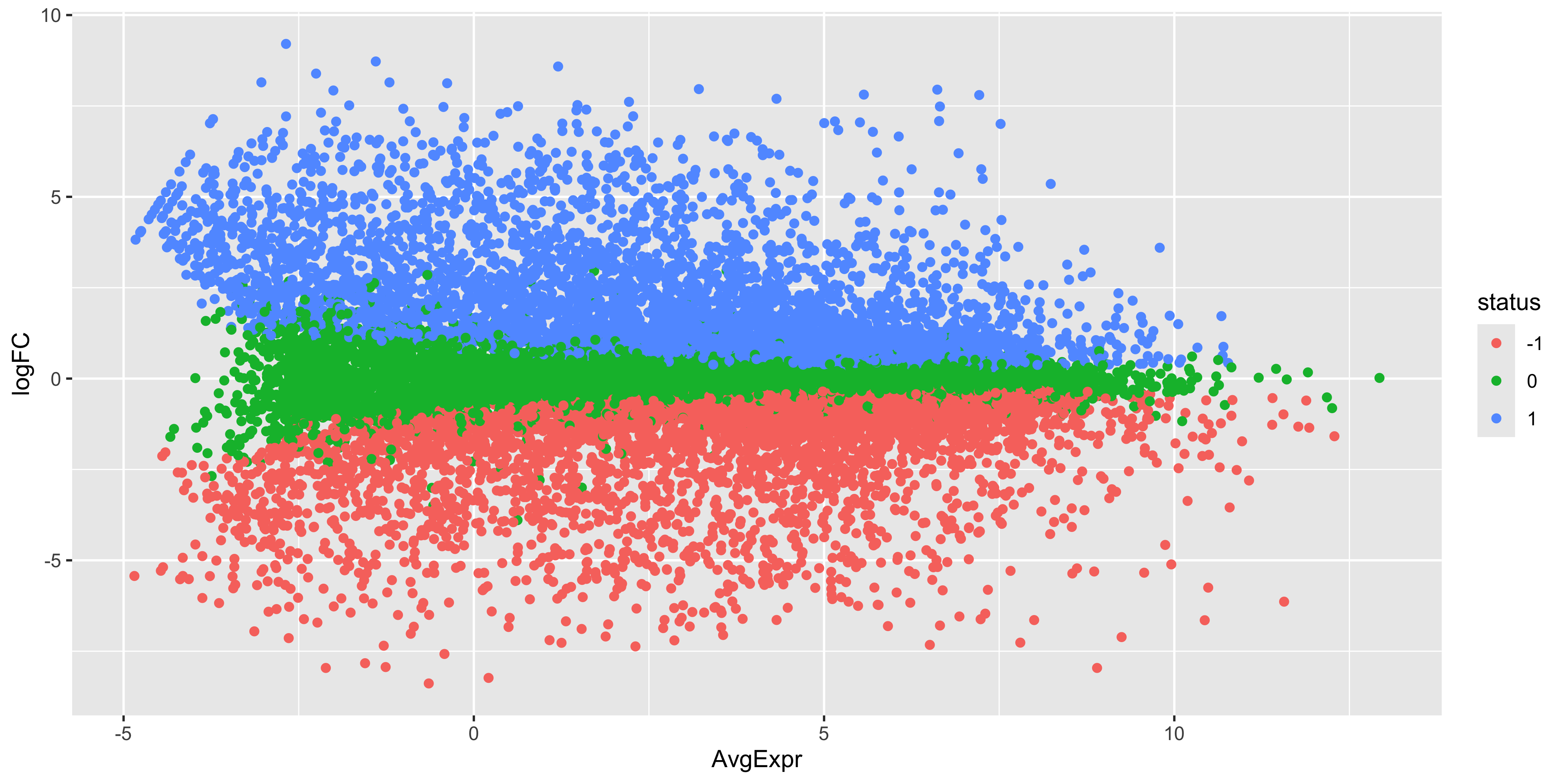
As before, we can try to re-create this plot using ggplot2 to give us more flexibility in plotting. The information we’ll need is the log-fold-change, the average log-expression and the differential expression status of each gene. We can extract this information from the efit and top data frame we created above, as well as gene names for annotation purposes.
With our tibble prepared, we can use ggplot2 to create the plot as we have done before
ma_plot_data %>%ggplot(aes(x = AvgExpr, y = logFC, col = status)) +geom_point()
While the coordinates of the points are the same, there is still quite a bit of work to do to make this plot look like the one produced by plotMA(). First we have the fix up the colours of the points. We also have to make it such that the non-significant points are plotted below the other points. To do this we would need to make it so that the non-significant points are plotted first. We can do this by reordering the levels of the status factor so that the non-significant points are plotted first. Labels can also be added using ggrepel for the top 15 most DE genes.
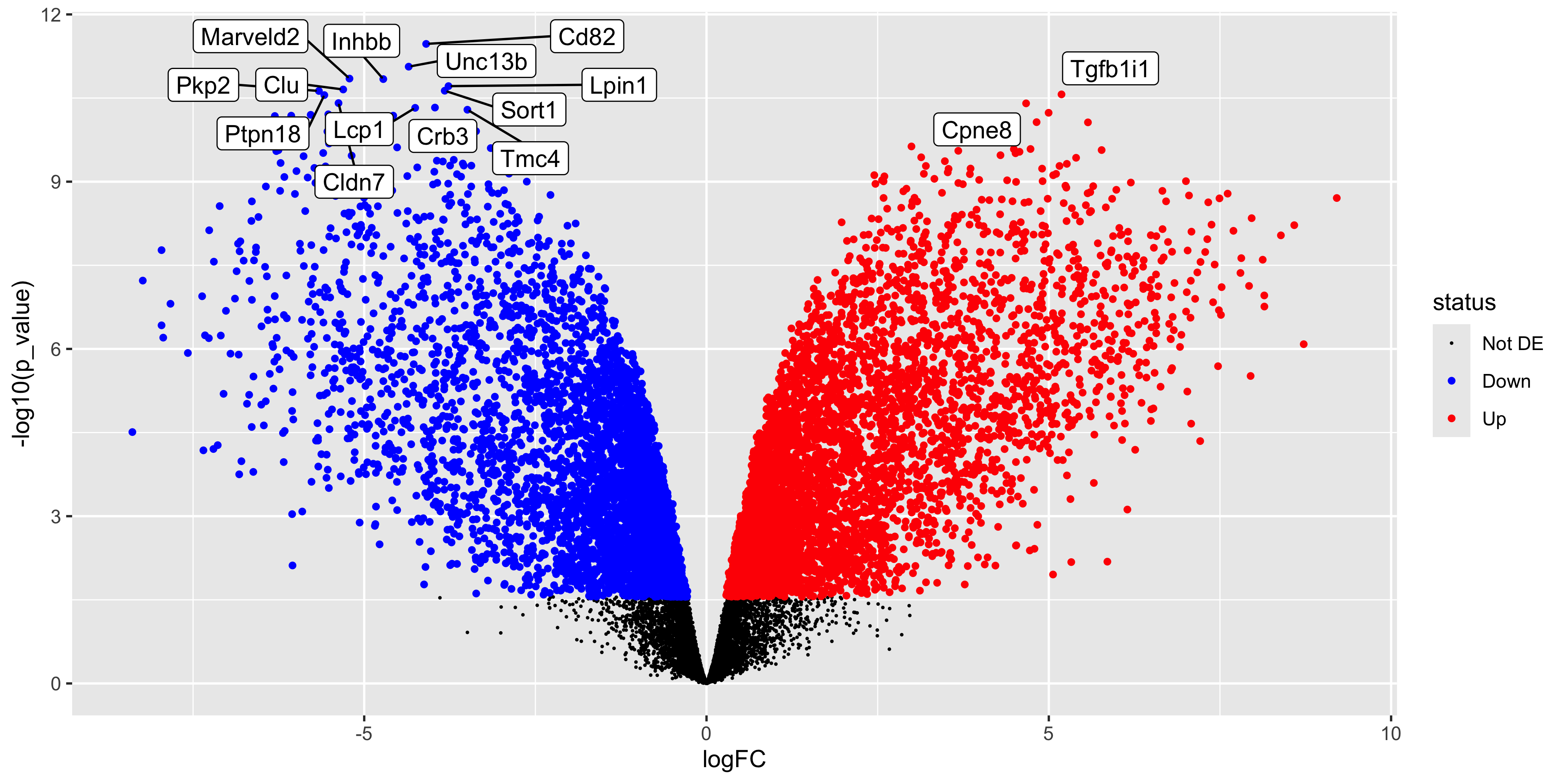
Since we have the tibble of the data prepared, we can also choose to create an alternative plot called a volcano plot. Which is also very popular in RNA-seq analysis. The volcano plot is a scatter plot of the negative log10 p-value against the log2 fold-change. This plot is useful for visualising the significance of the differentially expressed genes.
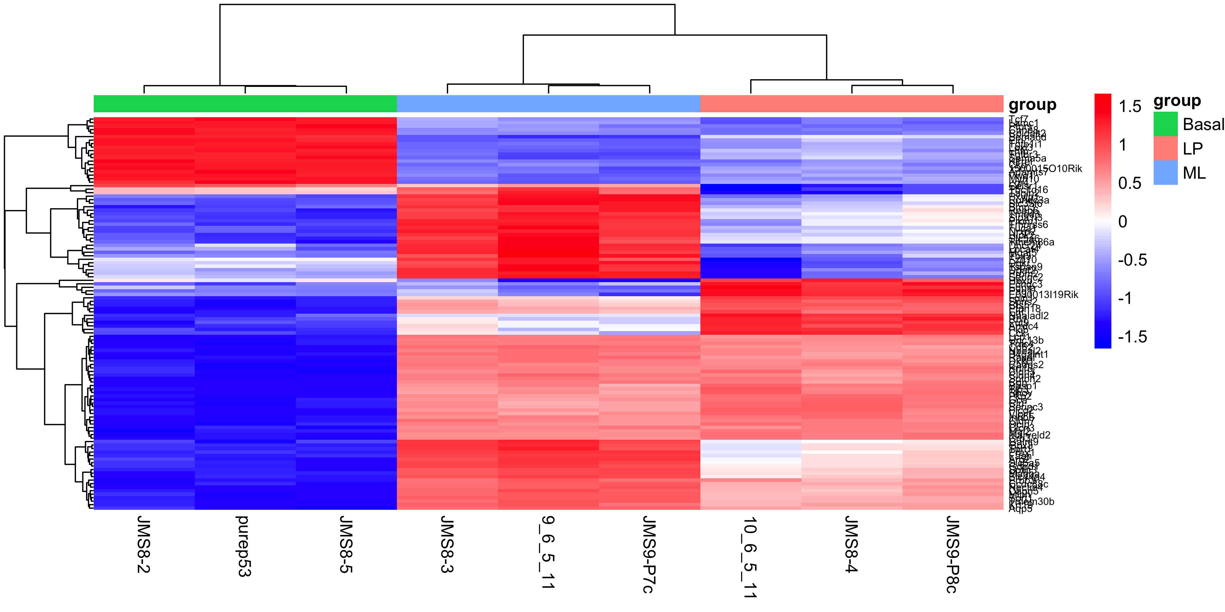
Finally we can create a heatmap of the differentially expressed genes. The heatmap is a useful way to visualise the expression of the differentially expressed genes across the samples. We can use the pheatmap package to create the heatmap.
First we need to install the package if you haven’t already
install.packages("pheatmap")
The data we will use for the heatmap is going to be the log2 cpm expression values of the top differentially expressed genes. We can use the topTable() function to get the top differentially expressed genes for each contrast. We can then use the cpm() function to get the expression values of these genes. We will take the top 50 genes from each contrast and combine them into a single data frame. We will then use extract the expression values for these genes from the full expression matrix. For more interpretable labels, we will use the gene symbols as the row names of the expression matrix.
Note that by default the ENTREZID column is encoded as a numeric value, so to use it to subset our expression matrix we need to convert it to a character vector in order to select the matching IDs rather than trying to select the numerical rows of the data.
top_genes <-bind_rows(topTable(efit, coef ="BasalvsLP", n =50),topTable(efit, coef ="BasalvsML", n =50),topTable(efit, coef ="LPvsML", n =50)) %>%select(ENTREZID, SYMBOL, TXCHROM) %>%distinct()top_gene_expr <-cpm(dge, log =TRUE)[as.character(top_genes$ENTREZID), ]rownames(top_gene_expr) <- top_genes$SYMBOL
To create the heatmap we will use the pheatmap() function with the expression matrix. We will add in arguments to provide our own colour scale, to scale the data along the rows with a z-score, adding in sample annotation and clustering the data by rows and columns. We will also add in the option to show the row names and column names, and set the font size of the row names. You can experiment with removing each of these options to see how they affect the heatmap, as well as investigate additional options in the pheatmap() documentation.
Now that we have produced a series of plots and the top genes table, we can save these files to a directory. These figures may form the basis for publication figures, and the results table can partially presented as a result, or the full table can be included as a supplementary file.
With that we have come to the conclusion of the RNA-seq analysis and this course. You have now learned how to use various tidyverse packages to operate on data and create publication quality figures. You have also learned how to use the limma and edgeR packages to perform differential expression analysis on RNA-seq data. You should now be able to apply these skills to perform analysis on your own data.
6.7 References
1.
Benjamini Y, Hochberg Y. Controlling the False Discovery Rate: A Practical and Powerful Approach to Multiple Testing. Journal of the Royal Statistical Society Series B: Statistical Methodology [Internet]. 1995 Jan 1;57(1):289–300. Available from: http://dx.doi.org/10.1111/j.2517-6161.1995.tb02031.x
Source Code
---filters: - naquizformat: html: toc: true toc-location: left toc-title: "In this session:"---# Session 6: RNA-seq part 2The aim of this session is to complete the analysis of the RNA-seq data using the `limma` and `edgeR` packages. With the results of the analysis, we want to be able to produce publication quality figures and write out the results to a file for sharing or publication.::: {.callout-tip title="Learning Objectives"}- fit a linear model to the data- construct design and contrast matrices for the linear model- model the mean-variance relationship of the data using the `voom()` function- perform statistical testing to identify differentially expressed genes- visualise the results using an MA plot- write out the results to a file:::```{r}# load required packageslibrary(tidyverse)library(edgeR)library(limma)group <-parse_factor(c("LP", "ML", "Basal", "Basal", "ML", "LP", "Basal", "ML", "LP"),levels =c("Basal", "LP", "ML"))samplenames <-c("10_6_5_11", "9_6_5_11", "purep53", "JMS8-2", "JMS8-3","JMS8-4", "JMS8-5", "JMS9-P7c", "JMS9-P8c")# create DGEList objectdge <-readDGE(dir(path ="data/counts", pattern ="GSM*"),path ="data/counts",columns =c(1, 3),group = group,labels = samplenames)# add gene annotation informationdge$genes <-read_tsv("data/Ses3_geneAnnot.tsv")# filter lowly expressed geneskeep <-filterByExpr(dge)dge <- dge[keep, ]# normalise the data for library size and RNA compositiondge <-calcNormFactors(dge, method ="TMM")```## Linear modellingTo identify differentially expressed genes from our normalised gene expression data, we will use the `limma` package to fit linear models to the genes. A linear model is a broad class of statistical models that fit the value of an response (or dependent) variable as a linear function of one or more explanatory (or independent) variables (also called covariates).The general form of a linear model looks like this:$Y = \beta_{0} + \beta_{1}X_{1} + \beta_{2}X_{2}... + \epsilon$This equation is saying that a response variable of interest $Y$ is equal to a constant ($\beta_{0}$) plus the sum of the covariates ($X_{i}$) each multiplied by a constant coefficient ($\beta_{i}$) and some error term ($\epsilon$). The error term is the difference between the observed value and the predicted value of the model and is assumed to have a normal distribution with mean 0 and some variance.Our experiment is quite simple, since there is only a single covariate, the cell type. The true benefit of using linear models is in its ability to accommodate more complex designs including multiple covariates.To fit the linear models in the limma-voom framework we need two objects in addition to our data:- A design matrix, representing the covariates.- A contrast matrix, representing the specific comparison we wish to make.### Design matrixThe first step to fitting a linear model is to specify a design matrix. The design matrix specifies the values of the covariates for each sample, and is represented as a matrix due to the mathematical convenience.To generate a design matrix. We use the function `model.matrix()`, with the expression `~0 + group`. This returns a matrix representing the design where there is no intercept term and group is the only covariate. If we omit the `0` then there would be an intercept in the model, and if we included more covariates then more columns would be generated.```{r}design <-model.matrix(~0+ group, data = dge$samples)design```There are 9 rows, one for each sample. Along the columns are the names of the groups. The values in the cells denote membership of the particular sample for a particular group, as our groups in this case are mutually exclusive, each row contains only a single 1 to denote membership in a single group.### ContrastsContrast matrices are companions to design matrices. They are used to specify the comparison of interest. In our case, we have three experimental groups: `Basal`, `LP` and `ML`. So if we are to perform differential expression analysis, we are most likely interested in the differences between only two of the groups at a time. Contrast matrices let use specify which comparison we'd like to make, and are also represented as a matrix just like the design.A contrast matrix can be made using the `makeContrasts()` function. Within this function, we specify the name of each specific contrast and the formula for that contrast. For example, the `BasalvsLP` contrasts compares the difference between the `Basal` and `LP` groups. Note that the name of the phenotype groups must be written exactly as they are in the column names of our design matrix (see above).In addition to the individual contrasts, the function must know about the design of the model. This is passed through the `levels` argument, which either accepts a matrix with the column names corresponding to levels of your experimental groups, or the levels themselves as a character vector. Here we first simplify the column names of our design matrix to make it easier to read. Then we create the contrast matrix using the `makeContrasts()` function.```{r}colnames(design) <-c("Basal", "LP", "ML")contr_matrix <-makeContrasts(BasalvsLP ="Basal - LP",BasalvsML ="Basal - ML",LPvsML ="LP - ML",levels = design # alternatively 'levels = colnames(design)')contr_matrix```There are two things to note about a design matrix. First, the sum of the numbers in each row is equal to 0. Second, the way that you set up the equation in the matrix will determine the interpretation of the log-fold-change calculated later, as well as the meaning of up-regulated and down-regulated genes. For example, the contrast `Basal - LP` will give a positive log-fold-change for genes that are up-regulated in the `Basal` group compared to the `LP` group. If we had set up the contrast as `LP - Basal`, then the opposite would be true, and we would get a negative log-fold-change for genes that are up-regulated in the `Basal` group compared to the `LP` group.### Variance modelling with voomWe are now ready to fit our linear models. Limma fits linear models to the data with the assumption that the underlying data is normally distributed. Count data is generally not normally distributed, but log transforming count data gives it a roughly normal distribution sufficient for linear models to work well. To do this, limma transforms the raw count data to log-cpm using library sizes and the normalisation factors we calculated previously.In addition to the normalisation steps, the limma-voom pipeline uses the `voom()` function to generate weights for the individual genes based on a modelled mean-variance relationship. This modelling allows use to get more information out of small sample sizes as the weights prevent our model from being more heavily influenced by more variable data points. The weights will then allow the linear model to be less influenced by genes with high variability, which is important for small sample sizes. The voom function also generates a mean-variance plot, which is useful for visualising the data.The `voom()` function takes as arguments, our `DGEList` object and our design matrix. It also optionally outputs a plot of the mean-variance relationship of our data, called the 'voom-plot'.```{r}v <-voom(dge, design, plot =TRUE)```The output of `voom()` (our variable `v`) is an `EList` object which contains the following elements:- `genes` - a data frame of gene annotation data.- `targets` - data frame of sample data.- `E` - numeric matrix of normalised log-cpm values.- `weights` - numeric matrix of precision weights.- `design` - the design matrix.The MA plot shows the mean-variance relationship of the data. The x-axis is the average log2 expression of each gene, and the y-axis is the log2 standard deviation of each gene. The idea is that the variance of a gene can be estimated as a function of its main expression, and that this estimate is more accurate than the direct calculation of the variance.### Fitting the linear modelWe are now ready to fit our linear model with `lmFit()`, which calculates coefficients we defined in our design matrix `design`. The resulting object, `vfit` is a `MArrayLM` object. It contains a information about our genes (the same data frame as `genes` from our `EList` object `v` above), the design matrix and a number of statistical outputs. Of most interest to us is the coefficients, stored in an element called `coefficients`. The first rows of this matrix is shown below. Each gene is row and is labelled using the EntrezID. Each column gives coefficients for each of our phenotype groups. These coefficients are weighted averages of the log-cpm of each gene in each group.```{r}vfit <-lmFit(v)head(vfit$coefficients)```We can then use `contrasts.fit()` to calculate coefficients for each contrast (or 'comparison') we specified in our `contr_matrix`. The output is also an object of the class `MArrayLM` (also known as an `MArrayLM` object). When we inspect the `coefficients` element now, we can see that each column is a contrast that we specified in our contrast matrix.```{r}vfit <-contrasts.fit(vfit, contrasts = contr_matrix)head(vfit$coefficients)```With these values we essentially want to know whether or not the difference in values is significantly different from 0. If the difference is not significantly different from 0, then we have failed to establish a difference in the expression of a particularly gene between two groups. If the difference is significantly greater than 0, then we have up-regulation in the first group of the contrast, and if the difference is significantly less than 0, then we have down-regulation in the first group of the contrast.## Statistical testingTo actually test if the values are significantly different from 0, we use the `eBayes()` function to compute moderated t-statistics, moderated F-statistics and log-odds of differential expression for each gene, given a fitted linear model. 'Moderated' refers to empirical Bayes moderation, which borrows information across genes to obtain more accurate measures of variability for each gene. This also increases our power to detect differentially expressed genes.```{r}efit <-eBayes(vfit)```We can now look at the number of differentially expressed genes using the `decideTests()` function. The output of this function is a matrix where each column is a contrast (comparison of interest) and each row is a gene. The numbers 1, -1 and 0 mean up-regulated, down-regulated or not significantly differentially expressed, respectively.Note that `decideTests()` also accounts for multiple testing. The default method is Benjamini and Hochberg [@benjamini1995] but several others are also available.```{r}dt <-decideTests(efit)dt```To obtain the total number of differentially expressed genes for each comparison, we can add the function `summary()`:```{r}summary(dt)```The function `topTable()` can be used to obtain more information on the differentially expressed genes for each contrast. `topTable()` takes as arguments the `MArrayLM` object output by `eBayes()` (`efit`), the contrast name of interest and the number of top differentially expressed genes to output. Note that the contrast name must be given in quotes and must be exactly as written in the contrast matrix `contr_matrix`.It outputs a data frame with the following information:- **Gene details** - gene information, from the `gene` element of the `MArrayLM` object (`efit`).- `logFC` - the log2 fold change of the contrast.- `AveExpr` - the average log2 expression of that gene.- `t` - moderated t-statistic.- `P.Value` - p value.- `adj.P.Val` - adjusted p value.- `B` - log-odds that the gene is differentially expressed.```{r}top <-topTable(efit, coef ="BasalvsLP", n =Inf)head(top)```## MA PlotThe MA plot is a plot of log-fold-change (M-values) against log-expression averages (A-values), this is a common plot in RNA sequencing analysis to visualise the result of differential expression tests. It can be created using the `plotMA()` from the `limma` package. Creating this plot requires 3 pieces of information:- `object = efit`: The the fitted object containing the log-fold-change and log-expression averages- `coef = 1`: The column number of the contrast to plot since there are 3 different contrasts fitted within the object.- `status = dt[, 1]`: A vector of numerics denoting whether a gene is up-regulated or down-regulated.```{r}plotMA(efit, coef =1, status = dt[, "BasalvsLP"])```As before, we can try to re-create this plot using `ggplot2` to give us more flexibility in plotting. The information we'll need is the log-fold-change, the average log-expression and the differential expression status of each gene. We can extract this information from the `efit` and `top` data frame we created above, as well as gene names for annotation purposes.```{r}ma_plot_data <-tibble(logFC = efit$coefficients[, "BasalvsLP"],AvgExpr = efit$Amean,status =factor(as.numeric(dt[, "BasalvsLP"])),gene = efit$genes$SYMBOL,p_value = efit$p.value[, "BasalvsLP"])```With our tibble prepared, we can use `ggplot2` to create the plot as we have done before```{r}ma_plot_data %>%ggplot(aes(x = AvgExpr, y = logFC, col = status)) +geom_point()```While the coordinates of the points are the same, there is still quite a bit of work to do to make this plot look like the one produced by `plotMA()`. First we have the fix up the colours of the points. We also have to make it such that the non-significant points are plotted below the other points. To do this we would need to make it so that the non-significant points are plotted first. We can do this by reordering the levels of the `status` factor so that the non-significant points are plotted first. Labels can also be added using `ggrepel` for the top 15 most DE genes.```{r}library(ggrepel)ma_plot_data_fct <- ma_plot_data %>%mutate(status =fct_recode( status,"Not DE"="0","Down"="-1","Up"="1" ) ) %>%mutate(status =fct_relevel(status, "Not DE", "Down", "Up"))top_de_genes <- ma_plot_data_fct %>%arrange(p_value) %>%slice_head(n =15)scale_cols <-c("Not DE"="black","Down"="blue","Up"="red")ma_plot <- ma_plot_data_fct %>%ggplot(aes(x = AvgExpr, y = logFC, col = status)) +geom_point(data = ma_plot_data_fct %>%filter(status =="Not DE"), size =0.1) +geom_point(data = ma_plot_data_fct %>%filter(status !="Not DE"), size =1) +geom_label_repel(data = top_de_genes,aes(label = gene, col =NULL),max.overlaps =20,show.legend =FALSE ) +scale_colour_manual(values = scale_cols)```## Volcano PlotSince we have the tibble of the data prepared, we can also choose to create an alternative plot called a volcano plot. Which is also very popular in RNA-seq analysis. The volcano plot is a scatter plot of the negative log10 p-value against the log2 fold-change. This plot is useful for visualising the significance of the differentially expressed genes.```{r}volcano_plot <- ma_plot_data_fct %>%ggplot(aes(x = logFC, y =-log10(p_value), col = status)) +geom_point(data = ma_plot_data_fct %>%filter(status =="Not DE"), size =0.1) +geom_point(data = ma_plot_data_fct %>%filter(status !="Not DE"), size =1) +geom_label_repel(data = top_de_genes,aes(label = gene, col =NULL),max.overlaps =20,show.legend =FALSE ) +scale_colour_manual(values =c("black", "blue", "red"))volcano_plot```## HeatmapFinally we can create a heatmap of the differentially expressed genes. The heatmap is a useful way to visualise the expression of the differentially expressed genes across the samples. We can use the `pheatmap` package to create the heatmap.First we need to install the package if you haven't already```{r, eval = FALSE}install.packages("pheatmap")```The data we will use for the heatmap is going to be the log2 cpm expression values of the top differentially expressed genes. We can use the `topTable()` function to get the top differentially expressed genes for each contrast. We can then use the `cpm()` function to get the expression values of these genes. We will take the top 50 genes from each contrast and combine them into a single data frame. We will then use extract the expression values for these genes from the full expression matrix. For more interpretable labels, we will use the gene symbols as the row names of the expression matrix.Note that by default the ENTREZID column is encoded as a numeric value, so to use it to subset our expression matrix we need to convert it to a character vector in order to select the matching IDs rather than trying to select the numerical rows of the data.```{r}top_genes <-bind_rows(topTable(efit, coef ="BasalvsLP", n =50),topTable(efit, coef ="BasalvsML", n =50),topTable(efit, coef ="LPvsML", n =50)) %>%select(ENTREZID, SYMBOL, TXCHROM) %>%distinct()top_gene_expr <-cpm(dge, log =TRUE)[as.character(top_genes$ENTREZID), ]rownames(top_gene_expr) <- top_genes$SYMBOL```To create the heatmap we will use the `pheatmap()` function with the expression matrix. We will add in arguments to provide our own colour scale, to scale the data along the rows with a z-score, adding in sample annotation and clustering the data by rows and columns. We will also add in the option to show the row names and column names, and set the font size of the row names. You can experiment with removing each of these options to see how they affect the heatmap, as well as investigate additional options in the `pheatmap()` documentation.```{r}library(pheatmap)sample_anno <- dge$samples %>%select(group)heatmap <-pheatmap( top_gene_expr,color =colorRampPalette(c("blue", "white", "red"))(100),scale ="row",annotation_col = sample_anno,border_color =NA,cluster_rows =TRUE,cluster_cols =TRUE,show_rownames =TRUE,show_colnames =TRUE,fontsize_row =6)```## Saving all the resultsNow that we have produced a series of plots and the top genes table, we can save these files to a directory. These figures may form the basis for publication figures, and the results table can partially presented as a result, or the full table can be included as a supplementary file.```{r, warning=FALSE}dir.create("output")write_csv(top, "output/top_genes_BasalvsLP.csv")ggsave("output/ma_plot_BasalvsLP.png", ma_plot)ggsave("output/volcano_plot_BasalvsLP.png", volcano_plot)ggsave("output/heatmap_BasalvsLP.png", heatmap$gtable)```With that we have come to the conclusion of the RNA-seq analysis and this course. You have now learned how to use various `tidyverse` packages to operate on data and create publication quality figures. You have also learned how to use the `limma` and `edgeR` packages to perform differential expression analysis on RNA-seq data. You should now be able to apply these skills to perform analysis on your own data.## References