---
filters:
- naquiz
format:
html:
toc: true
toc-location: left
toc-title: "In this session:"
---
# Session 2: Working with data {#sec-session02}
In this session we will learn how to manipulate and summarise data using the `dplyr` package (with a little help from the `tidyr` package too).
::: {.callout-tip title="Learning Objectives"}
At the end of this session, learners should be able to:
1. Use the pipe (`%>%`) to chain multiple functions together
2. Design chains of dplyr functions to manipulate data frames
3. Understand how to identify and handle missing values in a data frame
4. Apply grouping for more complex analysis of data
5. Recall how to save data frames to a file
:::
Both `dplyr` and `tidyr` are contained within the `tidyverse` (along with `readr`) so we can load all of these packages at once using `library(tidyverse)`:
```{r}
# don't forget to load tidyverse!
library(tidyverse)
```
## Chaining functions together with pipes {#sec-pipes}
Pipes are a powerful feature of the `tidyverse` that allow you to chain multiple functions together. Pipes are useful because they allow you to break down complex operations into smaller steps that are easier to read and understand.
For example, take the following code:
```{r}
my_vector <- c(1, 2, 3, 4, 5)
as.character(round(mean(my_vector)))
```
What do you think this code does? It calculates the mean of `my_vector`, rounds the result to the nearest whole number, and then converts the result to a character. But the code is a bit hard to read because you have to start from the inside of the brackets and work your way out.
Instead, we can use the pipe operator (`%>%`) to chain these functions together in a more readable way:
```{r}
my_vector <- c(1, 2, 3, 4, 5)
my_vector %>% mean() %>% round() %>% as.character()
```
See how the code reads naturally from left to right? You can think of the pipe as being like the phrase "and then". Here, we're telling R: "Take `my_vector`, and then calculate the mean, and then round the result, and then convert it to a character."
You'll notice that we didn't need to specify the input to each function. That's because the pipe automatically passes the output of the previous function as the first input to the next function. We can still specify additional arguments to each function if we need to. For example, if we wanted to round the mean to 2 decimal places, we could do this:
```{r}
my_vector %>% mean() %>% round(digits = 2) %>% as.character()
```
R is clever enough to know that the first argument to `round()` is still the output of `mean()`, even though we've now specified the `digits` argument.
::: {.callout-note title="Plenty of pipes"}
There is another style of pipe in R, called the 'base R pipe' `|>`, which is available in R version 4.1.0 and later. The base R pipe works in a similar way to the `magrittr` pipe (`%>%`) that we use in this course, but it is not as flexible. We recommend using the `magrittr` pipe for now.
Fun fact: the `magrittr` package is named after the [artist René Magritte, who made a famous painting of a pipe](https://en.wikipedia.org/wiki/The_Treachery_of_Images).
:::
To type the pipe operator more easily, you can use the keyboard shortcut {{< kbd Cmd-shift-M >}} (although once you get used to it, you might find it easier to type `%>%` manually).
::: {.callout-important title="Practice exercises"}
Try these practice questions to test your understanding
::: question
1\. What is NOT a valid way to re-write the following code using the pipe operator: `round(sqrt(sum(1:10)), 1)`. If you're not sure, try running the different options in the console to see which one gives the same answer.
::: choices
::: choice
`1:10 %>% sum() %>% sqrt() %>% round(1)`
:::
::: {.choice .correct-choice}
`sum(1:10) %>% sqrt(1) %>% round()`
:::
::: choice
`1:10 %>% sum() %>% sqrt() %>% round(digits = 1)`
:::
::: choice
`sum(1:10) %>% sqrt() %>% round(digits = 1)`
:::
:::
:::
::: question
2\. What is the output of the following code? `letters %>% head() %>% toupper()` Try to guess it before copy-pasting into R.
::: choices
::: choice
`"A" "B" "C" "D" "E" "F" "G" "H" "I" "J" "K" "L" "M" "N" "O" "P" "Q" "R" "S" "T" "U" "V" "W" "X" "Y" "Z"`
:::
::: choice
`"a" "b" "c" "d" "e" "f"`
:::
::: choice
An error
:::
::: {.choice .correct-choice}
`"A" "B" "C" "D" "E" "F"`
:::
:::
:::
<details>
<summary>Solutions</summary>
<p>
1. The invalid option is `sum(1:10) %>% sqrt(1) %>% round()`. This is because the `sqrt()` function only takes one argument, so you can't specify `1` as an argument in addition to what is being piped in from `sum(1:10)`. Note that some options used the pipe to send `1:10` to `sum()` (like `1:10 %>% sum()`), and others just used `sum(1:10)` directly. Both are valid ways to use the pipe, it's just a matter of personal preference.
2. The output of the code `letters %>% head() %>% toupper()` is `"A" "B" "C" "D" "E" "F"`. The `letters` vector contains the lowercase alphabet, and the `head()` function returns the first 6 elements of the vector. Finally, the `toupper()` function then converts these elements to uppercase.
</p>
</details>
:::
## Basic data manipulation {#sec-dataManip}
To really see the power of the pipe, we will use it together with the `dplyr` package that provides a set of functions to easily filter, sort, select, and summarise data frames. These functions are designed to work well with the pipe, so you can chain them together to create complex data manipulations in a readable format.
For example, even though we haven't covered the `dplyr` functions yet, you can probably guess what the following code does:
```{r}
#| eval: false
# use the pipe to chain together our data manipulation steps
dosage %>%
  filter(cage_number == "3E") %>%
  pull(weight_lost_g) %>%
  mean()
```
This code filters the `dosage` data frame to only include data from cage 3E, then pulls out the `weight_lost_g` column, and finally calculates the mean of the values in that column. The first argument to each function is the output of the previous function, and any additional arguments (like the column name in `pull()`) are specified in the brackets (like `round(digits = 2)` from the previous example).
We also used the enter key after each pipe `%>%` to break up the code into multiple lines to make it easier to read. This isn't required, but is a popular style in the R community, so all the code examples in this session will follow this format.
We will now introduce some of the most commonly used `dplyr` functions for manipulating data frames. To showcase these, we will use the `dosage` dataset that we practiced reading in last session. This imaginary dataset contains information on the weight lost by different strains of mice after being treated with different doses of MouseZempic®.
```{r}
# read in the data, like we did in session 1
dosage <- read_delim("data/mousezempic_dosage_data.csv")
```
Before we start, let's use what we learned in the previous session to take a look at `dosage`:
```{r}
dosage
```
You might also like to use `View()` to open the data in a separate window and get a closer look.
Taking a look at your data is the first, and one of the most important steps in analysis! It allows you to check that you're using the correct data file, and make sure that it was read into R correctly. Also, you might get some ideas of the first data manipulations you want to do, like filtering out certain rows or converting the units of a particular column.
::: {.callout-note title="Using RStudio autocomplete"}
A fun fact about bioinformaticians, we love to avoid typing as much as possible! It can be a pain to keep typing out the name of our dataset (even though `dosage` is pretty short), but luckily, RStudio has a handy autocomplete feature that can solve this problem. Just start typing the name of the object, and you'll see it will popup:
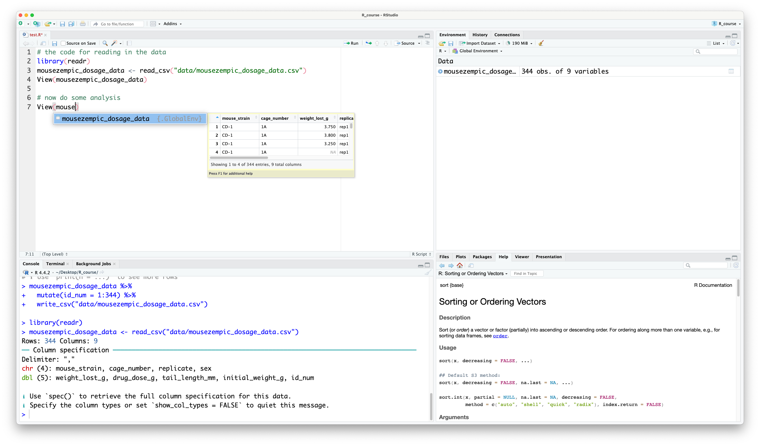
You can then press {{< kbd Tab >}} to autocomplete it. If there are multiple objects that start with the same letters, you can use the arrow keys to cycle through the options.
Try using autocomplete this session to save yourself some typing!
:::
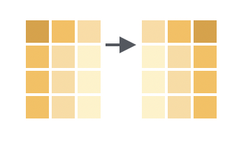
### Sorting data {#sec-sorting}
Sorting data is a great way to start to explore it. In `dplyr`, this is called 'arranging' and is done with the `arrange()` function.
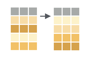
By default, `arrange()` sorts in ascending order (smallest values first). For example, let's sort the `dosage` data frame by the `weight_lost_g` column:
```{r}
dosage %>%
  arrange(weight_lost_g)
```
If we compare this to when we just printed our data above, we can see that the rows are now sorted so that the mice that lost the least weight are at the top. This allows us to investigate those particular mice and start to form the basis of research questions: for example, most of these mice are female, so does that mean that mousezempic is not as effective on female mice?
You might also want to sort in descending order (largest values first). You can do this by putting the `desc()` function around your column name, inside `arrange()`:
```{r}
dosage %>%
  # put desc() around the column name to sort in descending order
  arrange(desc(weight_lost_g))
```
Now we can see the mice that lost the most weight are at the top. What do you notice about these mice?
::: {.callout-note title="Comments and pipes"}
Notice how in the previous example we have written a comment in the middle of the pipe chain. This is a good practice to help you remember what each step is doing, especially when you have a long chain of functions, and won't cause any errors as long as you make sure that the comment is on its own line.
You can also write comments at the end of the line, just make sure it's after the pipe operator `%>%`.
For example, these comments are allowed:
```{r}
dosage %>% # a comment here is fine
  # a comment here is fine
  arrange(desc(weight_lost_g))
```
But this will cause an error, because the `#` is before the pipe, so R treats it as part of the comment (notice how the `%>%` has changed colour?) and doesn't know how the two lines relate to each other. It tries to run them separately, which for the first line is ok (it will just print `dosage`):
```{r}
#| error: true
dosage # this comment will cause an error %>%
arrange(desc(weight_lost_g))
```
But for the second line, there is an error that R doesn't know what the `weight_lost_g` object is. That's because it's a column in the `dosage` data frame, so R only knows what it is in the context of the pipe chain containing that data frame.
:::
You can also sort by multiple columns by passing multiple column names to `arrange()`. For example, to sort by the strain first and then by the amount of weight lost:
```{r}
# sort by strain first, then by weight lost
dosage %>%
  arrange(mouse_strain, weight_lost_g)
```
This will sort the data frame by strain (according to alphabetical order, as it is a character column), and within each strain, they are then sorted by the amount of weight lost.
::: {.callout-note title="Piping into View()"}
In the above example, we sorted the data by strain and then by weight lost, but because there are so many mice in each strain, the preview shown in our console doesn't allow us to see the full effect of the sorting.
One handy trick you can use with pipes is to add `View()` at the end of your chain to open the data in a separate window. Try running this code, and you'll be able to scroll through the full dataset to check that the other mouse strains have also been sorted correctly:
```{r}
#| eval: false
# sort by strain first, then by weight lost
dosage %>%
  arrange(mouse_strain, weight_lost_g) %>%
  View()
```
This is a great way to check that your code has actually done what you intended!
:::
#### Extracting rows with the smallest or largest values {#sec-sliceMinMax}
Slice functions are used to select rows based on their position in the data frame. The `slice_min()` and `slice_max()` functions are particularly useful, because they allow you to select the rows with the smallest or largest values in a particular column.
This is equivalent to using `arrange()` followed by `head()`, but is more concise:
```{r}
# get the 10 mice with the lowest drug dose
dosage %>%
  # slice_min() requires the column to sort by, and n = the number of rows to keep
  slice_min(drug_dose_g, n = 10)
# get the top 5 mice that lost the most weight
dosage %>%
  # slice_max() has the same arguments as slice_min()
  slice_max(weight_lost_g, n = 5)
```
But wait— neither of those pieces of code actually gave the number of rows we asked for! In the first example, we asked for the 10 mice with the lowest drug dose, but we got 13. And in the second example, we asked for the top 5 mice that lost the most weight, but we got 6. Why aren't the `slice_` functions behaving as expected?
If we take a look at the help page (type `?slice_min` in the console), we learn that `slice_min()` and `slice_max()` have an argument called `with_ties` that is set to `TRUE` by default. If we want to make sure we only get the number of rows we asked for, we would have to set it to `FALSE`, like so:
```{r}
# get the top 5 mice that lost the most weight
dosage %>%
  # no ties allowed!
  slice_max(weight_lost_g, n = 5, with_ties = FALSE)
```
This is an important lesson: sometimes functions will behave in a way that is unexpected, and you might need to read their help page or use other guides/google/AI to understand why.
::: {.callout-important title="Practice exercises"}
Try these practice questions to test your understanding
::: question
1\. Which code would you use to sort the `dosage` data frame from biggest to smallest initial weight?
::: choices
::: choice
`dosage %>% sort(initial_weight_g)`
:::
::: choice
`dosage %>% arrange(initial_weight_g)`
:::
::: choice
`dosage %>% sort(descending(initial_weight_g))`
:::
::: {.choice .correct-choice}
`dosage %>% arrange(desc(initial_weight_g))`
:::
:::
:::
::: question
2\. Which code would you use to extract the 3 mice with the highest initial weight from the `dosage` data frame?
::: choices
::: {.choice .correct-choice}
`dosage %>% slice_max(initial_weight_g, n = 3)`
:::
::: choice
`dosage %>% arrange(desc(initial_weight_g))`
:::
::: choice
`dosage %>% slice_min(initial_weight_g, n = 3)`
:::
::: choice
`dosage %>% arrange(initial_weight_g)`
:::
:::
:::
::: question
3\. I've written the below code, but one of the comments is messing it up! Which one?
```{r}
#| eval: false
# comment A
dosage # comment B %>%
  # comment C
  slice_max(weight_lost_g, n = 5, with_ties = FALSE) # comment D
```
::: choices
::: choice
Comment A
:::
::: {.choice .correct-choice}
Comment B
:::
::: choice
Comment C
:::
::: choice
Comment D
:::
:::
:::
<details>
<summary>Solutions</summary>
1. The correct code to sort the `dosage` data frame from biggest to smallest initial weight is `dosage %>% arrange(desc(initial_weight_g))`. The `arrange()` function is used to sort the data frame (although there is a `sort()` function in R, that's not part of dplyr and won't work the same way), and the `desc()` function is used to sort in descending order.
2. The correct code to extract the 3 mice with the highest initial weight from the `dosage` data frame is `dosage %>% slice_max(initial_weight_g, n = 3)`. The `slice_max()` function is used to select the rows with the largest values in the `initial_weight_g` column, and the `n = 3` argument specifies that we want to keep 3 rows. The `arrange()` function is not needed in this case, because `slice_max()` will automatically sort the data frame by the specified column.
3. The comment that is messing up the code is Comment B. The `#` symbol is before the pipe operator `%>%`, so R treats it as part of the comment and this breaks our chain of pipes. The other comments are fine, because they are either at the end of the line or on their own line. Basically, if a comment is changing the colour of the pipe operator (or any other bits of your code), it's in the wrong place!
</details>
:::
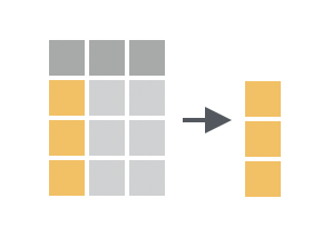
### Filtering data (rows) {#sec-filter}
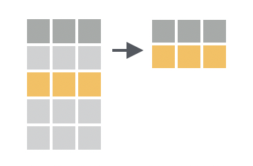
Filtering is useful not only as a way to explore our data, but also for answering a variety of analysis questions. In `dplyr`, the `filter()` function is used to subset rows based on their values. You provide a logical test, and `filter()` will keep the rows where the test is `TRUE`. We can write these tests using the comparison operators we learned in the previous session (e.g. `==`, `<` and `!=`, see [Section @sec-comparisons]).
For example, to filter the `dosage` data frame to only include mice that lost more than 6g:
```{r}
dosage %>%
  filter(weight_lost_g > 6)
```
Or to only include mice from cage 3E:
```{r}
dosage %>%
  # remember that == is used for testing equality
  filter(cage_number == "3E") # don't forget the quotes either!
```
#### Combining logical tests
Sometimes we want to filter based on multiple conditions. Here we will show some more advanced operators that can be used to combine logical tests.
The `&` operator is used to combine two logical tests with an 'and' condition. For example, to filter the data frame to only include mice that have a tail length greater than 19mm and are female:
```{r}
dosage %>%
  filter(tail_length_mm > 19 & sex == "female")
```
The `|` operator is used to combine two logical tests with an 'or' condition. For example, to filter the data frame to only include mice that have an initial weight less than 35g or a tail length less than 14mm:
```{r}
dosage %>%
  filter(initial_weight_g < 35 | tail_length_mm < 14)
```
The `%in%` operator can be used to filter based on a vector of multiple values (`c(x, y)`). It's particularly useful when you have a few character values you want to filter on, as it is shorter to type than `|` (or).
For example, to filter the data frame to only include mice from cages 3E or 1A, we could use `|` like this:
```{r}
dosage %>%
  filter(cage_number == "3E" | cage_number == "1A")
```
Or we could use `%in%` like this:
```{r}
dosage %>%
  filter(cage_number %in% c("3E", "1A"))
```
::: {.callout-important title="Practice exercises"}
Try these practice questions to test your understanding
::: question
1\. Which code would you use to filter the `dosage` data frame to only include mice from replicate 2?
::: choices
::: choice
`dosage %>% filter(replicate == 2)`
:::
::: choice
`dosage %>% filter(replicate == rep2)`
:::
::: {.choice .correct-choice}
`dosage %>% filter(replicate == "rep2")`
:::
::: choice
`dosage %>% filter(replicate = "rep2")`
:::
:::
:::
::: question
2\. What is NOT a valid way to filter the `dosage` data frame to only include mice that lost more than 4g, and have an initial weight less than 40g?
::: choices
::: choice
`dosage %>% filter(weight_lost_g > 4) %>% filter(initial_weight_g < 40)`
:::
::: {.choice .correct-choice}
`dosage %>% filter(weight_lost_g > 4) %>% (initial_weight_g < 40)`
:::
::: choice
`dosage %>% filter(weight_lost_g > 4 & initial_weight_g < 40)`
:::
::: choice
`dosage %>% filter(initial_weight_g < 40) %>% filter(weight_lost_g > 4)`
:::
:::
:::
::: question
3\. Which option correctly describes what the following code is doing?
```{r}
#| eval: false
dosage %>%
  filter(mouse_strain %in% c("BALB C", "Black 6")) %>%
  filter(weight_lost_g > 3 & weight_lost_g < 5) %>%
  arrange(desc(drug_dose_g))
```
::: choices
::: choice
Filters the data frame to remove mice from the "BALB C" and "Black 6" strains, who only lost between 3 and 5g of weight, and then sorts the data frame by drug dose.
:::
::: choice
Filters the data frame to remove mice from the "BALB C" and "Black 6" strains, that lost between 3 and 5g of weight, and then sorts the data frame by drug dose in descending order.
:::
::: choice
Filters the data frame to only include mice from the "BALB C" and "Black 6" strains, that lost between 3 and 5g of weight, and then sorts the data frame by drug dose.
:::
::: {.choice .correct-choice}
Filters the data frame to only include mice from the "BALB C" and "Black 6" strains, that lost between 3 and 5g of weight, and then sorts the data frame by drug dose in descending order.
:::
:::
:::
<details>
<summary>Solutions</summary>
1. The correct code to filter the `dosage` data frame to only include mice from replicate 2 is `dosage %>% filter(replicate == "rep2")`. Option A is incorrect because `2` is not a value of `replicate` (when filtering you need to know what values are actually in your columns! So make sure to `View()` your data first). Option B is incorrect because the replicate column is a character column, so you need to use quotes around the value you are filtering on. Option D is incorrect because `=` is not the correct way to test for equality, you need to use `==`.
2. The invalid option is `dosage %>% filter(weight_lost_g > 4) %>% (initial_weight_g < 40)`. This is because the second filtering step is missing the name of the filter function, so R doesn't know what to do with `(initial_weight_g < 40)`. The other options are valid ways to filter the data frame based on the specified conditions; note that we can use multiple `filter()` functions in a row to apply multiple conditions, or the `&` operator to combine them into a single `filter()` function. It's just a matter of personal preference.
3. The correct description of the code is that it filters the data frame to only include mice from the "BALB C" and "Black 6" strains, then filters those further to only those that lost between 3 and 5g of weight, and finally sorts the data frame by drug dose in descending order.
</details>
:::
### Dealing with missing values {#sec-missing}
Missing values are a common problem in real-world datasets. In R, missing values are represented by `NA`. In fact, if you look at the `dosage` data frame we've been using, you'll see that some of the cells contain `NA`: try spotting them with the `View()` function.
You can also find missing values in a data frame using the `is.na()` function in combination with `filter()`. For example, to find all the rows in the `dosage` data frame that have a missing value for the `drug_dose_g` column:
```{r}
dosage %>%
  filter(is.na(drug_dose_g))
```
The problem with missing values is that they can cause problems when you try to perform calculations on your data. For example, if you try to calculate the mean of a column that contains even a single missing value, the result will also be `NA`:
```{r}
# try to calculate the mean of the drug_dose_g column
# remember from session 1 that we can use $ to access columns in a data frame
dosage$drug_dose_g %>% mean()
```
`NA` values in R are therefore referred to as 'contagious': if you put an `NA` in you usually get an `NA` out. If you think about it, that makes sense— when we don't know the value of a particular mouse's drug dose, how can we calculate the average? That missing value could be anything.
For this reason, it's important to deal with missing values before performing calculations. Many functions in R will have an argument called `na.rm` that you can set to `TRUE` to remove missing values before performing the calculation. For example, to calculate the mean of the `drug_dose_g` column with the missing values excluded:
```{r}
# try to calculate the mean of the drug_dose_g column
# remember from session 1 that we can use $ to access columns in a data frame
dosage$drug_dose_g %>% mean(na.rm = TRUE)
```
This time, the result is a number, because the missing values have been removed before the calculation.
But not all functions have an `na.rm` argument. In these cases, you can remove rows with missing values. This can be done for a single column, using the `filter()` function together with `is.na()`:
```{r}
# remove rows with missing values in the drug_dose_g column
dosage %>%
  # remember the ! means 'not', it negates the result of is.na()
  filter(!is.na(drug_dose_g))
```
Or, you can remove rows with missing values in any column using the `na.omit()` function:
```{r}
# remove rows with missing values in any column
dosage %>%
  na.omit()
```
Sometimes, instead of removing rows with missing values, you might want to replace them with a specific value. This can be done using the `replace_na()` function from the `tidyr` package. `replace_na()` takes a `list()` which contains each of the column names you want to edit, and the value that should be used.
For example, to replace missing values in the `weight_lost_g` columns with 0, replace missing values in the `sex` column with 'unknown' and leave the rest of the data frame unchanged:
```{r}
# replace missing values in the drug_dose_g column with 0
dosage %>%
  # here we need to provide the column_names = values_to_replace
  # this needs to be contained within a list()
  replace_na(list(weight_lost_g = 0, sex = "unknown"))
```
When deciding how to handle missing values, you might have prior knowledge that `NA` should be replaced with a specific value, or you might decide that removing rows with `NA` is the best approach for your analysis.
For example, maybe we knew that the mice were given a `weight_lost_g` of `NA` if they didn't lose any weight, it would then make sense to replace those with 0 (as we did in the code above). However, if the `drug_dose_g` column was missing simply because the data was lost, we might choose to remove those rows entirely.
It's important to think carefully about how missing values should be handled in your analysis.
::: {.callout-important title="Practice exercises"}
Try these practice questions to test your understanding
::: question
1\. What would be the result of running this R code: `mean(c(1, 2, 4, NA))`
::: choices
::: choice
2.333333
:::
::: choice
0
:::
::: {.choice .correct-choice}
`NA`
:::
::: choice
An error
:::
:::
:::
::: question
2\. Which line of code would you use to filter the `dosage` data frame to remove mice that have a missing value in the `tail_length_mm` column?
::: choices
::: choice
`dosage %>% filter(tail_length_mm != NA)`
:::
::: choice
`dosage %>% filter(is.na(tail_length_mm))`
:::
::: choice
`dosage %>% na.omit()`
:::
::: {.choice .correct-choice}
`dosage %>% filter(!is.na(tail_length_mm))`
:::
:::
:::
::: question
3\. How would you replace missing values in the `initial_weight_g` column with the value 35?
::: choices
::: {.choice .correct-choice}
`dosage %>% replace_na(list(initial_weight_g = 35))`
:::
::: choice
`dosage %>% replace_na(initial_weight_g = 35)`
:::
::: choice
`dosage %>% replace_na(list(initial_weight_g == 35))`
:::
::: choice
`dosage %>% replace_na(35)`
:::
:::
:::
<details>
<summary>Solutions</summary>
<p>
1. The result of running the code `mean(c(1, 2, 4, NA))` is `NA`. This is because the `NA` value is 'contagious', so when you try to calculate the mean of a vector that contains an `NA`, the result will also be `NA`. If we wanted to calculate the mean of the vector without the `NA`, we would need to use the `na.rm = TRUE` argument.
2. The correct line of code to filter the `dosage` data frame to remove mice that have a missing value in the `tail_length_mm` column is `dosage %>% filter(!is.na(tail_length_mm))`. The `!` symbol is used to negate the result of `is.na()`, so we are filtering to keep the rows where `tail_length_mm` is not `NA`. We can't use the first option with the `!= NA` because `NA` is a special value in R that represents missing data, and it can't be compared to anything, and the third option is incorrect because `na.omit()` removes entire rows with missing values, rather than just filtering based on a single column.
3. The correct line of code to replace missing values in the `initial_weight_g` column with the value 35 is `dosage %>% replace_na(list(initial_weight_g = 35))`. The `replace_na()` function takes a `list()` that contains the column names you want to replace and the values you want to replace them with. We only need to use a single equal sign here as we're not testing for equality, we're assigning a value.
</p>
</details>
:::
### Selecting columns {#sec-select}
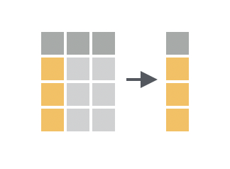
While `filter()` is used to subset rows, `select()` is used to subset columns. You can use `select()` to keep only the columns you're interested in, or to drop columns you don't need. This makes it easier to focus on just part of the dataset, so you can answer a particular analysis question.
The `select()` function takes the names of the columns that you want to keep/remove (no vector notation `c()` or quotation marks `""` necessary). For example, to select only the `mouse_strain`, `initial_weight_g`, and `weight_lost_g` columns from the `dosage` data frame:
```{r}
dosage %>%
  select(mouse_strain, initial_weight_g, weight_lost_g)
```
We can see that all the other columns have been removed from the data frame.
If you want to keep all columns except for a few, you can use `-` to drop columns. For example, to keep all columns except for `cage_number` and `sex`:
```{r}
dosage %>%
  select(-cage_number, -sex)
```
There are also some helper functions that can be used to select columns based on their names :
+-----------------+---------------------------------------------------+-------------------------------------------------+
| Function | Description | Example |
+=================+===================================================+=================================================+
| `starts_with()` | select column(s) that start with a certain string | select all columns starting with the letter i |
| | | |
| | | `select(starts_with("i"))` |
+-----------------+---------------------------------------------------+-------------------------------------------------+
| `ends_with()` | select column(s) that end with a certain string | select all columns ending with \_g |
| | | |
| | | `select(ends_with("_g"))` |
+-----------------+---------------------------------------------------+-------------------------------------------------+
| `contains()` | select column(s) that contain a certain string | select all columns containing the word 'weight' |
| | | |
| | | `select(contains("weight"))` |
+-----------------+---------------------------------------------------+-------------------------------------------------+
: There are several helper functions that can be used with the select function
Note that you need to use quotation marks around the arguments in these helper functions, as they aren't full column names, just strings of characters. These functions make it easier to write code that is more generic and can be re-used across multiple datasets (for example, if you used the `select(ends_with("_g"))` code from the table above, you could select all of the columns measured in grams, and convert those to kg or mg, regardless of what the full column name is).
Try using these helper functions to select columns from the `dosage` data frame!
::: {.callout-note title="Reordering columns"}
 We can reorder columns using the `relocate()` function, which works similarly to `select()` (except it just moves columns around rather than dropping/keeping them). For example, to move the `sex` column to before the `cage_number` column:
```{r}
dosage %>%
  # first the name of the column to move, then where it should go
  relocate(sex, .before = cage_number)
```
Two useful helper functions here are the `everything()` and `last_col()` functions, which can be used to move columns to the start/end of the data frame.
```{r}
# move id_num to the front
dosage %>%
  relocate(id_num, .before = everything()) # don't forget the brackets
# move mouse_strain to the end
dosage %>%
  relocate(mouse_strain, .after = last_col())
```
Re-ordering columns isn't necessary, but it makes it easier to see the data you're most interested in within the console (since often not all of the columns will fit on the screen at once). For example, if we are doing a lot of computation on the `initial_weight_g` column, we'd probably like to have that near the start so we can easily check it.
:::
Note that the output of the `select()` function is a new data frame, even if you only select a single column:
```{r}
# select the mouse_strain column
dosage %>%
  select(mouse_strain) %>%
  # recall from session 1 that class() tells us the type of an object
  class()
```
Sometimes, we instead want to get the values of a column as a vector.
We can do this by using the `pull()` function, which extracts ('pulls out') a single column from a data frame as a vector:
```{r}
# get the mouse_strain column as a vector
dosage %>%
  pull(mouse_strain) %>%
  class()
```
We can see that the class of the output is now a vector, rather than a data frame. This is important because some functions only accept vectors, not data frames, like `mean()` for example:
```{r}
# this will give an error
dosage %>% select(initial_weight_g) %>% mean(na.rm = TRUE)
# this will work
dosage %>% pull(initial_weight_g) %>% mean(na.rm = TRUE)
```
Note how both times we used `na.rm = TRUE` to remove missing values before calculating the mean.
You might remember that we used the `$` operator in the previous session to extract a single column from a data frame, so why use `pull()` instead? The main reason is that `pull()` works within a chain of pipes, whereas `$` doesn't.
For example, let's say we want to know the average initial weight of mice that lost at least 4g. We can do this by chaining `filter()` and `pull()` together:
```{r}
dosage %>%
  # filter to mice that lost at least 4g
  filter(weight_lost_g >= 4) %>%
  # get the initial_weight_g column as a vector
  pull(initial_weight_g) %>%
  # calculate mean, removing NA values
  mean(na.rm = TRUE)
```
::: {.callout-important title="Practice exercises"}
Try these practice questions to test your understanding
::: question
1\. Which line of code would NOT be a valid way to select the `drug_dose_g`, `initial_weight_g`, and `weight_lost_g` columns from the `dosage` data frame?
::: choices
::: choice
`dosage %>% select(drug_dose_g, initial_weight_g, weight_lost_g)`
:::
::: {.choice .correct-choice}
`dosage %>% select(contains("g"))`
:::
::: choice
`dosage %>% select(ends_with("_g"))`
:::
::: choice
`dosage %>% select(-cage_number, -tail_length_mm, -id_num, -mouse_strain, -sex, -replicate)`
:::
:::
:::
::: question
2\. How would I extract the `initial_weight_g` column from the `dosage` data frame as a vector?
::: choices
::: choice
`dosage %>% filter(initial_weight_g)`
:::
::: choice
`dosage %>% $initial_weight_g`
:::
::: choice
`dosage %>% select(initial_weight_g)`
:::
::: {.choice .correct-choice}
`dosage %>% pull(initial_weight_g)`
:::
:::
:::
::: question
3\. How would you move the `sex` column to the end of the `dosage` data frame?
::: choices
::: choice
`dosage %>% relocate(sex)`
:::
::: choice
`dosage %>% relocate(sex, .after = last_col)`
:::
::: {.choice .correct-choice}
`dosage %>% relocate(sex, .after = last_col())`
:::
::: choice
`dosage %>% reorder(sex, .after = last_col())`
:::
:::
:::
<details>
<summary>Solutions</summary>
<p>
1. The line of code that would NOT be a valid way to select the `drug_dose_g`, `initial_weight_g`, and `weight_lost_g` columns from the `dosage` data frame is `dosage %>% select(contains("g"))`. This line of code would select all columns that contain the letter 'g', which would include columns like `cage_number` and `tail_length_mm`. We need to specify either `ends_with("g")` or `contains("_g")` to only get those with `_g` at the end. The other options are valid ways to select the specified columns, although some are more efficient than others!
2. The correct way to extract the `initial_weight_g` column from the `dosage` data frame as a vector is `dosage %>% pull(initial_weight_g)`. The `pull()` function is used to extract a single column from a data frame as a vector. The other options are incorrect because `filter()` is used to subset rows, `$` is not used in a pipe chain, and `select()` is outputs a data frame, not extract them as vectors.
3. The correct way to move the `sex` column to the end of the `dosage` data frame is using the `relocate()` function like this: `dosage %>% relocate(sex, .after = last_col())`. The `last_col()` function is used to refer to the last column in the data frame. The other options are incorrect because `reorder()` is not a valid function, and you need to remember to include the brackets `()` when using `last_col()`.
</p>
</details>
:::
### Modifying data {#sec-mutate}
So far, we've learned how to filter rows and select columns from a data frame. But what if we want to change the data itself? This is where the `mutate()` function comes in.
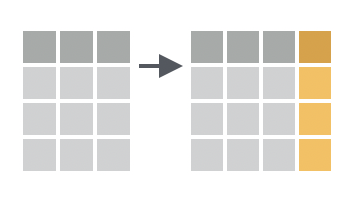
The `mutate()` function is used to add new columns to a data frame, or modify existing columns, often by performing some sort of calculation. For example, we can add a new column to `dosage` that contains the drug dose in mg (rather than g):
```{r}
dosage %>%
  # add a new column called drug_dose_mg
  # convert drug_dose_g to mg by multiplying by 1000
  mutate(drug_dose_mg = drug_dose_g * 1000) %>%
  # just select the drug dose columns so we can compare them
  select(drug_dose_g, drug_dose_mg)
```
You can see that the `drug_dose_mg` column has been added to the data frame, and it contains, for each row, the value of the `drug_dose_g` column multiplied by 1000 (`NA` values are preserved).
These calculations can be as complex as you like, and involve multiple different columns. For example, to add a new column to the `dosage` data frame that calculates the weight lost as a percentage of the initial weight:
```{r}
dosage %>%
  # calculate the % of initial weight that was lost
  mutate(weight_lost_percent = (weight_lost_g / initial_weight_g) * 100)
```
A useful helper function for `mutate()` is the `case_when()` function, which allows you to create new columns based on multiple conditions. We do this with the notation `case_when(condition1 ~ value1, condition2 ~ value2, ...)`.
For example, to add a new column to the `dosage` data frame that categorises the mice based on how much weight they lost:
```{r}
dosage %>%
  # create a new column called weight_loss_category
  mutate(weight_loss_category = case_when(
    weight_lost_g < 4 ~ "Low", # separate conditions with a comma
    weight_lost_g <= 5 ~ "Medium",
    weight_lost_g > 5 ~ "High"
  )) %>%
  select(weight_lost_g, weight_loss_category)
```
Note that the conditions are evaluated in order, and the first condition that is `TRUE` is the one that is used. So if a mouse lost 4.5g, it `case_when()` would first test if it fits the 'Low' category (by checking if 4.5 is less than 4, which it isn't), and then if it fits the 'Medium' category (by checking if 4.5 is less than or equal to 5). Since it is, the mouse would be categorised as 'Medium'.
::: {.callout-note title="Fallback with default value(s)"}
In the above example, what would happen if a mouse lost -1g (gained weight)? It wouldn't fit any of the conditions, so it would get an `NA` in the `weight_loss_category` column. Sometimes you might want this behaviour, but other times you would prefer to specify a 'fallback' category that will be assigned to everything that doesn't fit in the other categories. You can do this by including a `.default =` argument at the end of the `case_when()` function. For example:
```{r}
dosage %>%
  # create a new column called weight_loss_category
  mutate(weight_loss_category = case_when(
    weight_lost_g < 4 ~ "Low", # separate conditions with a comma
    weight_lost_g <= 5 ~ "Medium",
    weight_lost_g > 5 ~ "High",
    .default = "Unknown"
  )) %>%
  select(weight_lost_g, weight_loss_category)
```
Notice how the `NA` value in the fourth row is now categorised as 'Unknown'.
:::
One final thing to note is that `mutate()` can be used to modify existing columns as well as add new ones. To do this, just use the name of the existing column as the 'new' one.
For example, let's use `mutate()` together with `case_when()` to modify the `sex` column so that it uses `M` and `F` instead `male` and `female`:
```{r}
dosage %>%
  # modify sex column
  mutate(sex = case_when(
    sex == "female" ~ "F",
    sex == "male" ~ "M",
    # if neither, code it as 'X'
    .default = "X"))
```
::: {.callout-important title="Practice exercises"}
Try these practice questions to test your understanding
::: question
1\. What line of code would you use to add a new column to the `dosage` data frame that converts the `tail_length_mm` column to cm?
::: choices
::: choice
`dosage %>% create(tail_length_cm = tail_length_mm / 10)`
:::
::: choice
`dosage %>% mutate(tail_length_cm == tail_length_mm / 10)`
:::
::: {.choice .correct-choice}
`dosage %>% mutate(tail_length_cm = tail_length_mm / 10)`
:::
::: choice
`dosage %>% tail_length_cm = tail_length_mm / 10`
:::
:::
:::
::: question
2\. Explain in words what the following code does:
```{r}
#| eval: false
dosage %>%
  arrange(desc(weight_lost_g)) %>%
  mutate(weight_lost_rank = row_number())
```
Hint: the row_number() function returns the number of each row in the data frame (1 being the first row and so on).
::: choices
::: choice
Adds a new column to the data frame that ranks the mice based on how much weight they lost, with 1 being the mouse that lost the least weight.
:::
::: {.choice .correct-choice}
Adds a new column to the data frame that ranks the mice based on how much weight they lost, with 1 being the mouse that lost the most weight.
:::
::: choice
Adds a new column to the data frame that ranks the mice
:::
::: choice
Does nothing, because the `row_number()` function has no arguments
:::
:::
:::
::: question
3\. What is wrong with this R code?
```{r}
#| error: true
dosage %>%
  mutate(weight_lost_category = case_when(
    weight_lost_g < 4 ~ "Low"
    weight_lost_g <= 5 ~ "Medium"
    weight_lost_g > 5 ~ "High"
  ))
```
::: choices
::: choice
You didn't include a `.default =` condition at the end of the `case_when()` function to act as a fallback
:::
::: choice
You can't use the `case_when()` function with the `mutate()` function
:::
::: choice
`weight_lost_g` is not a valid column name
:::
::: {.choice .correct-choice}
You need to separate the conditions in the `case_when()` function with a comma
:::
:::
:::
::: question
4\. Explain in words what the following code does:
```{r}
#| eval: false
dosage %>%
  mutate(mouse_strain = case_when(
    mouse_strain == "Black 6" ~ "B6",
    .default = mouse_strain
  ))
```
Hint: if you're not sure, try running the code, but pipe it into `View()` so that you can take a good look at what's happening in the `mouse_strain` column.
::: choices
::: choice
Renames the strains of all the mice to "B6", regardless of their original strain
:::
::: choice
This code will produce an error
:::
::: choice
Adds a new column that categorises the mice based on their strain, so that any mice from the "Black 6" strain are now called "B6", and all other strains are left unchanged.
:::
::: {.choice .correct-choice}
Modifies the `mouse_strain` column so that any mice from the "Black 6" strain are now called "B6", and all other strains are left unchanged.
:::
:::
:::
<details>
<summary>Solutions</summary>
<p>
1. The correct line of code to add a new column to the `dosage` data frame that converts the `tail_length_mm` column to cm is `dosage %>% mutate(tail_length_cm = tail_length_mm / 10)`.
2. The code `dosage %>% arrange(desc(weight_lost_g)) %>% mutate(weight_lost_rank = row_number())` adds a new column to the data frame that ranks the mice based on how much weight they lost, with 1 being the mouse that lost the most weight. First, the `arrange(desc(weight_lost_g))` function sorts the data frame by the `weight_lost_g` column in descending order, and then the `mutate(weight_lost_rank = row_number())` function adds a new column that assigns a rank to each row based on its position (row number) in the sorted data frame.
3. The error is that the conditions in the `case_when()` function are not separated by commas. Each condition should be followed by a comma because these are like the arguments in a function. Remeber that it's optional to include the `.default =` condition at the end of the `case_when()` function.
4. The code `dosage %>% mutate(mouse_strain = case_when(mouse_strain == "Black 6" ~ "B6", .default = mouse_strain))` modifies the `mouse_strain` column so that any mice from the "Black 6" strain are now called "B6", and all other strains are left unchanged. As we are calling our column `mouse_strain`, no new column is being created (we are modifying the existing one) and the `.default = mouse_strain` condition acts as a fallback to keep the original values (that already exist in the `mouse_strain` column) for any rows that don't match our first condition (strain being "Black 6").
</p>
</details>
:::
### Summarising data {#sec-summarise}
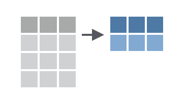
The `summarise()` (or `summarize()`, if you prefer US spelling) function is used to calculate summary statistics on your data. It takes similar arguments to `mutate()`, but instead of adding a new column to the data frame, it returns a new data frame with a single row and one column for each summary statistic you calculate.
For example, to calculate the mean weight lost by the mice in the `dosage` data frame:
```{r}
dosage %>%
  summarise(mean_weight_lost = mean(weight_lost_g, na.rm = TRUE))
```
We can also calculate multiple summary statistics at once. For example, to calculate the mean, median, and standard deviation of the weight lost by the mice:
```{r}
dosage %>%
  summarise(
    mean_weight_lost = mean(weight_lost_g, na.rm = TRUE),
    median_weight_lost = median(weight_lost_g, na.rm = TRUE),
    sd_weight_lost = sd(weight_lost_g, na.rm = TRUE)
  )
```
The power of summarising data is really seen when combined with grouping, which we will cover in the next section.
::: {.callout-important title="Practice exercises"}
Try these practice questions to test your understanding
::: question
1\. Explain in words what the following code does:
```{r}
#| eval: false
dosage %>%
  summarise(average_tail = mean(tail_length_mm, na.rm = TRUE),
            min_tail = min(tail_length_mm, na.rm = TRUE),
            max_tail = max(tail_length_mm, na.rm = TRUE))
```
::: choices
::: choice
Calculates the average, minimum, and maximum tail length of the mice in the `dosage` data frame.
:::
::: {.choice .correct-choice}
Produces a data frame containing one column for each of the average, minimum, and maximum tail length of the mice in the `dosage` data frame.
:::
::: choice
Finds the average tail length of the mice in the `dosage` data frame.
:::
::: choice
Produces a vector containing the average, minimum, and maximum tail length of the mice in the `dosage` data frame.
:::
:::
:::
::: question
2\. What is NOT a valid way to calculate the mean weight lost by the mice in the `dosage` data frame?
::: choices
::: choice
`dosage %>% summarise(mean_weight_lost = mean(weight_lost_g, na.rm = TRUE))`
:::
::: choice
`dosage %>% pull(weight_lost_g) %>% mean(na.rm = TRUE)`
:::
::: choice
`dosage %>% summarize(mean_weight_lost = mean(weight_lost_g, na.rm = TRUE))`
:::
::: {.choice .correct-choice}
`dosage %>% mean(weight_lost_g, na.rm = TRUE)`
:::
:::
:::
<details>
<summary>Solutions</summary>
1\. The code **produces a data frame** containing one column for each of the average, minimum, and maximum tail length of the mice in the `dosage` data frame.
2\. The line of code that is NOT a valid way to calculate the mean weight lost by the mice in the `dosage` data frame is `dosage %>% mean(weight_lost_g, na.rm = TRUE)`. This line of code is incorrect because the `mean()` function is being used directly on the data frame, rather than within a `summarise()` function. The other options are valid ways to calculate the mean weight lost by the mice in the `dosage` data frame (although note that the second option uses `pull()` to extract the `weight_lost_g` column as a vector before calculating the mean, so the mean value is stored in a vector rather than in a data frame).
</details>
:::
## Grouping {#sec-grouping}
Grouping is a powerful concept in in `dplyr` that allows you to perform operations on subsets of your data. For example, you might want to calculate the mean weight lost by mice in each cage, or find the mouse with the longest tail in each strain.
We can group data using the `.by` argument that exists in many dplyr functions, like `summarise()` and `mutate()`, and passing it the name(s) of column(s) to group by. For example, to calculate the mean weight lost by mice in each cage:
```{r}
dosage %>%
  summarise(
    mean_weight_lost = mean(weight_lost_g, na.rm = TRUE),
    # don't forget it's .by, not by!
    .by = cage_number)
```
Like when we first learned the summarise function above, we give our new column a name (`mean_weight_lost`), and then we assign its value to be the mean of the `weight_lost_g` column (with `NA`s removed). But this time, we also added the `.by` argument to specify the column we want to group by (`cage_number`, in this case). This will return a data frame with the mean weight lost by mice in each cage.
Grouping is a powerful tool for exploring your data and can help you identify patterns that might not be obvious when looking at the data as a whole. For example, notice how this grouped summary reveals that mice in cage 3E lost more weight than those in the other two cages.
It's also possible to group by multiple columns by passing a vector of column names to the `.by` argument. For example, to calculate the mean weight lost by mice in each cage and strain:
```{r}
dosage %>%
  summarise(mean_weight_lost = mean(weight_lost_g, na.rm = TRUE),
  # group by both cage_number and mouse_strain
    .by = c(cage_number, mouse_strain))
```
Of course, `mean()` is not the only function that we can use within `summarise()`. We can use any function that takes a vector of values and returns a single value, like `median()`, `sd()`, or `max()`. We can also use multiple functions at once, by giving each column a name and specifying the function we want to use:
```{r}
dosage %>%
  summarise(
    n = n(),
    mean_weight_lost = mean(weight_lost_g, na.rm = TRUE),
    median_weight_lost = median(weight_lost_g, na.rm = TRUE),
    sd_weight_lost = sd(weight_lost_g, na.rm = TRUE),
    max_weight_lost = max(weight_lost_g, na.rm = TRUE),
    min_weight_lost = min(weight_lost_g, na.rm = TRUE),
    .by = cage_number)
```
Here, we also used the `n()` function to calculate the number of mice in each cage. This is a special helper function that works within `summarise` to count the number of rows in each group.
::: {.callout-note title="To `.by` or not to `.by`?"}
In the `dplyr` package, there are two ways to group data: using the `.by` argument within various functions (as we have covered so far), or using the `group_by()` function, then performing your operations and ungrouping with `ungroup()`.
For example, we've seen above how to calculate the mean weight lost by mice in each cage using the `.by` argument:
```{r}
dosage %>%
  summarise(mean_weight_lost = mean(weight_lost_g, na.rm = TRUE), .by = cage_number)
```
But we can also do the same using `group_by()` and `ungroup()`:
```{r}
dosage %>%
  group_by(cage_number) %>%
  summarise(mean_weight_lost = mean(weight_lost_g, na.rm = TRUE)) %>%
  ungroup()
```
The two methods are equivalent, but using the `.by` argument within functions can be more concise and easier to read. Still, it's good to be aware of `group_by()` and `ungroup()` as they are widely used, particularly in older code.
:::
Although grouping is most often used with `summarise()`, it can be used with `dplyr` functions too. For example mutate() function can also be used with grouping to add new columns to the data frame based on group-specific calculations. Let's say we wanted to calculate the Z-score (also known as the [standard score](https://en.wikipedia.org/wiki/Standard_score)) to standardise the weight lost by each mouse within each strain.
As a reminder, the formula for calculating the Z-score is $\frac{x - \mu}{\sigma}$, where $x$ is the value (in our case the `weight_lost_g` column), $\mu$ is the mean, and $\sigma$ is the standard deviation.
We can calculate this for each mouse in each strain using the following code:
```{r}
dosage %>%
  # remove NAs before calculating the mean and SD
  filter(!is.na(weight_lost_g)) %>%
  mutate(weight_lost_z = (weight_lost_g - mean(weight_lost_g)) / sd(weight_lost_g), .by = mouse_strain) %>%
  # select the relevant columns
  select(mouse_strain, weight_lost_g, weight_lost_z)
```
Unlike when we used `.by` with `summarise()`, we still get the same number of rows as the original data frame, but now we have a new column `weight_lost_z` that contains the Z-score for each mouse within each strain. This could be useful for identifying outliers or comparing the weight lost by each mouse to the average for its strain.
::: {.callout-important title="Practice exercises"}
Try these practice questions to test your understanding
::: question
1\. Which line of code would you use to calculate the median tail length of mice belonging to each strain in the `dosage` data frame?
::: choices
::: choice
`dosage %>% summarise(median_tail_length = median(tail_length_mm), .by = mouse_strain)`
:::
::: {.choice .correct-choice}
`dosage %>% summarise(median_tail_length = median(tail_length_mm, na.rm = TRUE), .by = mouse_strain)`
:::
::: choice
`dosage %>% summarise(median_tail_length = median(tail_length_mm, na.rm = TRUE), by = mouse_strain)`
:::
::: choice
`dosage %>% mutate(median_tail_length = median(tail_length_mm, na.rm = TRUE), .by = mouse_strain)`
:::
:::
:::
::: question
2\. Explain in words what the following code does:
```{r}
#| eval: false
dosage %>%
  summarise(max_tail_len = max(tail_length_mm, na.rm = TRUE), .by = c(mouse_strain, replicate))
```
::: choices
::: choice
Calculates the maximum tail length of all mice for each strain in the `dosage` data frame
:::
::: choice
Calculates the maximum tail length of all mice for each replicate in the `dosage` data frame
:::
::: choice
Calculates the maximum tail length of all mice in the `dosage` data frame
:::
::: {.choice .correct-choice}
Calculates the maximum tail length of mice in each unique combination of strain and replicate in the `dosage` data frame.
:::
:::
:::
::: question
3\. I want to count how many male and how many female mice there are for each strain in the `dosage` data frame. Which line of code would I use?
::: choices
::: choice
`dosage %>% summarise(count = n(), .by = sex)`
:::
::: choice
`dosage %>% summarise(count = n(), .by = mouse_strain)`
:::
::: {.choice .correct-choice}
`dosage %>% summarise(count = n(), .by = c(mouse_strain, sex))`
:::
::: choice
`dosage %>% summarise(count = n(), .by = mouse_strain, sex)`
:::
:::
:::
::: question
4\. I want to find the proportion of weight lost **by each mouse** in each cage in the `dosage` data frame. Which line of code would I use?
::: choices
::: choice
`dosage %>% summarise(weight_lost_proportion = weight_lost_g / sum(weight_lost_g, na.rm = TRUE), .by = cage_number)`
:::
::: {.choice .correct-choice}
`dosage %>% mutate(weight_lost_proportion = weight_lost_g / sum(weight_lost_g, na.rm = TRUE), .by = cage_number)`
:::
::: choice
`dosage %>% mutate(weight_lost_proportion = weight_lost_g / sum(weight_lost_g, na.rm = TRUE, .by = cage_number))`
:::
::: choice
`dosage %>% mutate(weight_lost_proportion = weight_lost_g / sum(weight_lost_g, na.rm = TRUE))`
:::
:::
:::
<details>
<summary>Solutions</summary>
<p>
1. The correct line of code to calculate the median tail length of mice belonging to each strain in the `dosage` data frame is `dosage %>% summarise(median_tail_length = median(tail_length_mm, na.rm = TRUE), .by = mouse_strain)`. Remember to use `na.rm = TRUE` to remove any missing values before calculating the median, and to use `.by` to specify the column to group by (not `by`). Seeing as we want to calculate the median (collapse down to a single value per group), we need to use `summarise()` rather than `mutate()`.
2. The code `dosage %>% summarise(max_tail_len = max(tail_length_mm, na.rm = TRUE), .by = c(mouse_strain, replicate))` calculates the maximum tail length of mice in each **unique combination** of strain and replicate in the `dosage` data frame.
3. The correct line of code to count how many male and how many female mice there are for each strain in the `dosage` data frame is `dosage %>% summarise(count = n(), .by = c(mouse_strain, sex))`. We need to group by both `mouse_strain` and `sex` to get the count for each unique combination of strain and sex. Don't forget that we specify the column names as a vector when grouping by multiple columns.
4. The correct line of code to find the proportion of weight lost **by each mouse** in each cage in the `dosage` data frame is `dosage %>% mutate(weight_lost_proportion = weight_lost_g / sum(weight_lost_g, na.rm = TRUE), .by = cage_number)`. We use `mutate()` because we want a value for each mouse (each row in our data), rather than to collapse down to a single value for each group (cage number in this case). Be careful that you use the `.by` argument within the `mutate()` function call, not within the `sum()` function by mistake (this is what is wrong with the third option).
</p>
</details>
:::
## Saving data to a file {#sec-saving}
Once you've cleaned and transformed your data, you'll often want to save it to a file so that you can use it in other programs or share it with others. The `write_csv()` and `write_tsv()` functions from the `readr` package are a great way to do this. They take two arguments - the data frame you want to save and the file path where you want to save it.
For example, let's say I want to save my summary table of the weight lost by mice in each cage to a CSV file called `cage_summary_table.csv`:
```{r}
#| eval: false
# create the summary table
# and assign it to a variable
cage_summary_table <- dosage %>%
  summarise(
    n = n(),
    mean_weight_lost = mean(weight_lost_g, na.rm = TRUE),
    median_weight_lost = median(weight_lost_g, na.rm = TRUE),
    sd_weight_lost = sd(weight_lost_g, na.rm = TRUE),
    .by = cage_number)

# save the data to a CSV file
write_csv(cage_summary_table, "cage_summary_table.csv")
```
CSV files are particularly great because they can be easily read into other software, like Excel.
It's also possible to use the `write_*()` functions along with a pipe:
```{r}
#| eval: false
dosage %>%
  summarise(
    n = n(),
    mean_weight_lost = mean(weight_lost_g, na.rm = TRUE),
    median_weight_lost = median(weight_lost_g, na.rm = TRUE),
    sd_weight_lost = sd(weight_lost_g, na.rm = TRUE),
    .by = cage_number) %>%
  write_csv("cage_summary_table.csv")
```
Remember here that the first argument (the data frame to save) is passed on by the pipe, so the only argument in the brackets is the second one: the file path.
## Summary
Here's what we've covered in this session:
- The pipe operator `%>%` and how we can use it to chain together multiple function calls, making our code more readable and easier to understand.
- The basic dplyr verbs `filter()`, `select()`, `mutate()`, and `arrange()` and how they can be used to tidy and analyse data.
- Missing values (`NA`) and how to remove or replace them
- The `summarise()` function and how it can be used to calculate summary statistics on your data, as well as the power of grouping data with the `.by` argument.
::: {.callout-note title="Why does data need to be tidy anyway?"}
In this session, we've been focusing on manipulating our data to make it 'tidy': that is, structured in a consistent way that makes it easy to work with. A nice visual illustration of tidy data and its importance can be [found here](https://allisonhorst.com/other-r-fun), and we will cover the idea of tidy data in more detail in @sec-session04.
:::
### Practice questions
1. What is the purpose of the pipe operator `%>%`? Keeping this in mind, re-write the following code to use the pipe.
a. `round(mean(c(1, 2, 3, 4, 5)))`
b. `print(as.character(1 + 10))`
2. What would be the result of evaluating the following expressions? You don't need to know these off the top of your head, use R to help! (Hint: some expressions might give an error. Try to think about why)
a. `dosage %>% filter(weight_lost_g > 10)`
b. `dosage %>% select(tail_length_mm, weight_lost_g)`
c. `dosage %>% mutate(weight_lost_kg = weight_lost_g / 1000)`
d. `dosage %>% arrange(tail_length_mm)`
e. `dosage %>% filter(initial_Weight_g > 10) %>% arrange(mouse_strain)`
f. `dosage %>% relocate(mouse_strain, .after = cage_number)`
g. `dosage %>% pull(weight_lost_g)`
h. `dosage %>% filter(!is.na(weight_lost_g))`
i. `dosage %>% replace_na(list(weight_lost_g = 0))`
j. `dosage %>% summarise(mean_weight_lost = mean(weight_lost_g, na.rm = TRUE))`
k. `dosage %>% summarise(mean_weight_lost = mean(weight_lost_g, na.rm = TRUE), .by = cage_number)`
3. What is a missing value in R? What are two ways to deal with missing values in a data frame?
4. I want to add a new column to the `dosage` data frame that converts the `mouse_strain` column to lowercase. Hint: you can use the `tolower()` function in R to convert characters to lowercase. Look up its help page by typing `?tolower` in the R console to see how to use it.
5. How could you find the maximum tail length for each unique combination of sex and mouse strain in the `dosage` data frame?
6. Write a line of code to save the result of Q5 to a CSV file called `max_tail_length.csv`.
<details>
<summary>Solutions</summary>
1. The pipe operator `%>%` is used to chain together multiple function calls, passing the result of one function to the next. Here's how you could re-write the code to use the pipe:
a. `c(1, 2, 3, 4, 5) %>% mean() %>% round()`
b. `as.character(1 + 10) %>% print()`
2. The result of evaluating the expressions would be:
a. A data frame containing only the rows where `weight_lost_g` is greater than 10.
b. A data frame containing only the `tail_length_mm` and `weight_lost_g` columns.
c. A data frame with an additional column `weight_lost_kg` that contains the weight lost in kilograms.
d. A data frame sorted by `tail_length_mm`, in ascending order.
e. An error because `initial_Weight_g` is not a column in the data frame.
f. A data frame with the `mouse_strain` column moved to be after the `cage_number` column.
g. A **vector** containing the values of the `weight_lost_g` column.
h. A data frame containing only the rows where `weight_lost_g` is not `NA`.
i. A data frame with missing values in the `weight_lost_g` column replaced with 0.
j. A data frame with the mean weight lost by all mice.
k. A data frame with the mean weight lost by mice in each cage.
3. A missing value in R is represented by `NA`. Two ways to deal with missing values in a data frame are to remove them using `filter(!is.na(column_name))` or to replace them with a specific value using `replace_na(list(column_name = value))`.
4. To add a new column to the `dosage` data frame that converts the `mouse_strain` column to lowercase, you can use `mutate()` as follows\`:
```{r}
dosage %>%
  mutate(mouse_strain_lower = tolower(mouse_strain))
```
5. You can use the `max()` function within `summarise(.by = c(sex, mouse_strain))` to find the maximum tail length of each unique sex/mouse strain combination:
```{r}
dosage %>%
  summarise(max_tail_length = max(tail_length_mm, na.rm = TRUE), .by = c(sex, mouse_strain))
```
6. To save the result of Q5 to a CSV file called `max_tail_length.csv`, you can use the `write_csv()` function, either by using a pipe to connect it to the code you wrote previously:
```{r}
#| eval: false
dosage %>%
  summarise(max_tail_length = max(tail_length_mm, na.rm = TRUE), .by = c(sex, mouse_strain)) %>%
  write_csv("max_tail_length.csv")
```
Or by assigning this result to a variable and then saving it to a file:
```{r}
#| eval: false
max_tail_length <- dosage %>%
  summarise(max_tail_length = max(tail_length_mm, na.rm = TRUE), .by = c(sex, mouse_strain))

write_csv(max_tail_length, "max_tail_length.csv")
```
</details>


 We can reorder columns using the


