NAb-seq bioinformatics tutorial (old)

Introduction

EDIT 7/11/2022: This page explains how to run the old v0.1 of NAb-seq. We highly recommend you use NAb-seq v0.2 if possible (see top of page for an updated tutorial)

Welcome to the NAb-seq bioinformatics tutorial! This document will explain in detail how to generate high-accuracy antibody consensus sequences from whole-transcriptome nanopore sequencing data, as explained in the NAb-seq paper. An end-to-end script that covers all of the steps is available from the NAb-seq github repository, but going step-by-step is helpful for better understanding the process and troubleshooting.

The following figure summarises the steps of the NAb-seq workflow: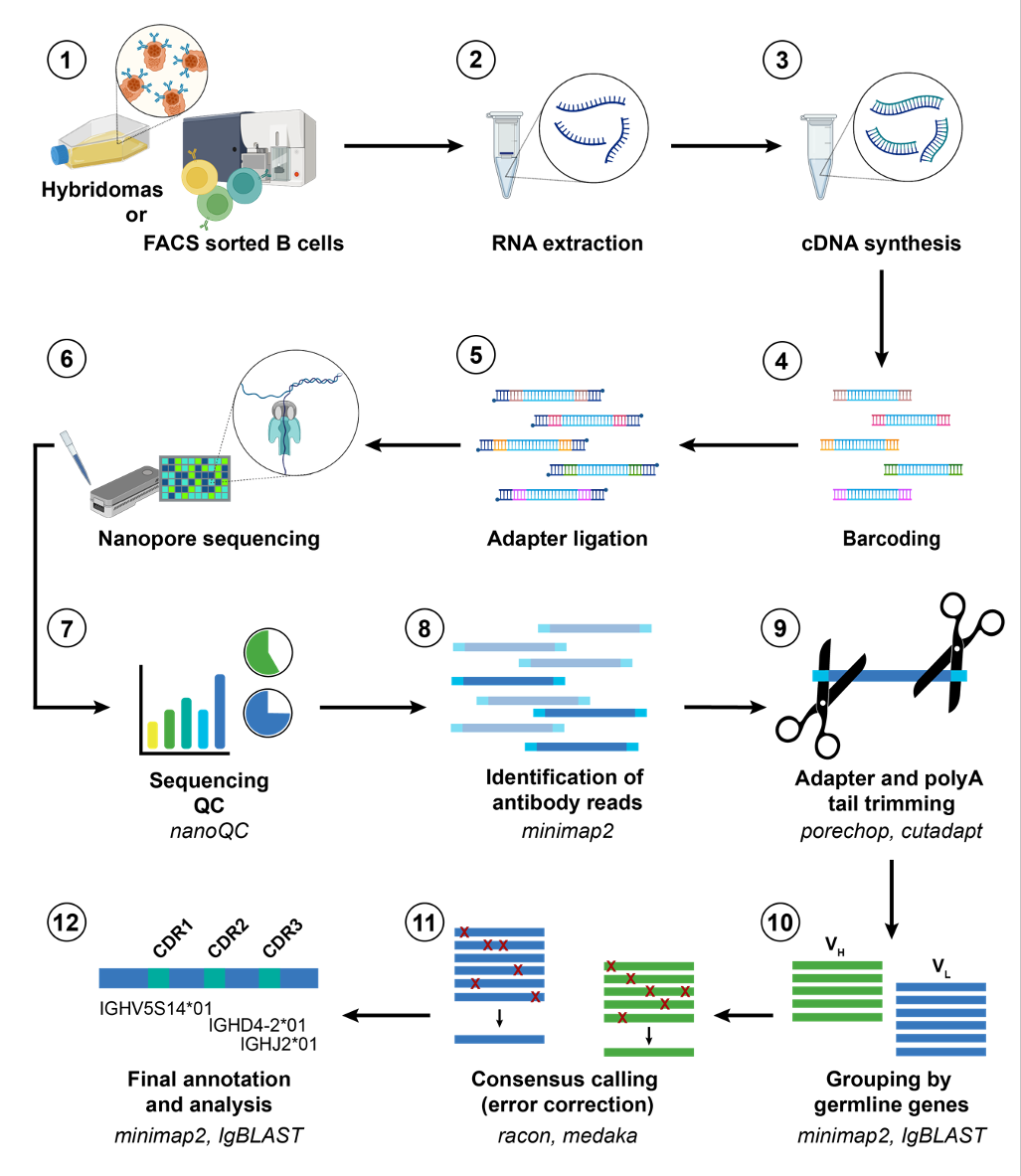

(since this is a bioinformatics tutorial, we will start from step 7, the sequencing QC)

Software required

The NAb-seq bioinformatics tutorial uses the following software:

NanoComp (optional, for QC purposes only)
minimap2 (for identification of antibody reads, and annotation of constant regions)
cutadapt (for trimming of adapters & polyA tails)
SeqKit (for manipulation of sequence files)
IgBLAST (for annotation of variable regions)
Racon (for consensus calling/error correction)
Medaka (for consensus calling/error correction)
R/RStudio (for processing the output of various tools & analysing the results)
- tidyverse packages will need to be installed

As each tool is required during the analysis process, installation instructions are provided. Alternatively, detailed instructions for installing and using each of the tools can be found at the links above.

Input files

Before beginning, it is important to prepare the necessary input files. These are:

Basecalled and demultiplexed ‘pass’ fastq files. These files come from running nanopore’s guppy basecalling tool, and should have names like barcode1_pass.fq.gz
- Basecalling means converting reads from raw signal into nucleotide sequences
- Demultiplexing means bioinformatically separating reads based on the barcodes added during library preparation
- Pass reads are reads that have an average quality above a certain cutoff (for nanopore super-high accuracy reads, this is a Q score of 10, or about 90% accuracy)
Constant gene reference fasta file. This should be a fasta format file containing the sequences of all constant genes for your organism of interest. In the NAb-seq github repository, files for rat and mouse are provided. To ensure you have the most up-to-date information, or to make files for another organism, these reference sequences can be retrieved from the IMGT website. See the appendix for detailed instructions on how to prepare the reference files.
Variable AND constant gene reference fasta file. This file should be the same as above, except that it should include the V(D)J variable region genes as well as the constant ones.
Sequencing summary .txt file. This is a file generated during sequencing, and it contains information about the reads (e.g. length, quality, number). This file is optional: it is required only for the quality control (QC) process.

In this tutorial, we will use as an example the reads from library A (representing the 7D10 antibody sequence). More information about this sample and how it was generated can be found in the NAb-seq paper. This data can be downloaded from the European Nucleotide Archive (ENA), under accession number PRJEB51442. To follow this tutorial, download the file named library_A.fq.gz. The following code assumes that your library_A.fq.gz file is located within a folder called input_data.

Quality control (QC)

Quality control (QC) is an important first step in bioinformatic workflows. QC tools can give us an idea of how well the sequencing run worked, in terms of the number of reads, what their quality (accuracy) is and how long they are. There are a number of tools for QC of nanopore sequencing data, but here we will use NanoComp.

QC with NanoComp

NanoComp is written in python, and can be installed via pip using the command: pip install NanoComp.

Once installed, the QC can be run as follows from within the tutorial folder:

# make a folder to store the QC results
mkdir qc

# run NanoComp
NanoComp --threads 4 --outdir qc --prefix "hybridomas" --barcoded --summary input_data/sequencing_summary_AGG119_0904ab6e.txt.gz

Where:

--threads 4 is the number of threads
--outdir qc tells NanoComp to put its output in the qc folder
--prefix "hybridomas" is the name we want to give this QC report
--barcoded tells NanoComp that our sequencing run is barcoded, so it will compare the various QC metrics across barcodes
--summary tells NanoComp the location of our sequencing summary file (change this to reflect your own sequencing summary file)

This command will produce a range of output files. These include:

hybridomasNanoComp-report.html which is report that will open in any web browser, containing all of the QC plots
hybridomasNanoComp-data.tsv.gz which is a file that contains the raw QC data used to make the plots. This can be useful if you want to do further analysis or make figures for a publication
A range of .png files of each of the individual plots

When looking at the results, the most important metric is the number of reads per barcode. A minimum of at least 40,000 reads per barcode is recommended. Below this number, the number of antibody transcripts may be insufficient to generate highly-accurate consensus sequences. If you are trying to detect the presence of additional productive heavy/light chains (which may have a low abundance (Bradbury et al. 2018)), then the more reads the better.

Identification of antibody reads

Once we have verified that the sequencing run went ok, the next step is to identify antibody reads. We will do this by aligning all of our reads (which represent the whole transcriptome) to the IMGT antibody reference sequences described in the input files section. The alignment tool (minimap2) will output a file describing all of the alignments it found between our reads and the antibody reference sequences. We will process this file in R to get a list of all candidate antibody reads, and then extract these from the main file using SeqKit.

Aligning reads to the antibody reference sequences

If you don’t have it already, you will first need to install minimap2. This is easiest through conda (more information about setting up conda can be found here). You can simply run the command conda install -c bioconda minimap2. Alternatively, it is available to download from github.

Running minimap2 is straightforward:

# make a folder to store the results of this step
mkdir identifying_ab_reads

# run minimap2
minimap2 -x map-ont -n 4 \
reference_sequences/imgt_rattus_norvegicus_refs.fasta \
inputdata/library_A_pass.fq.gz > \
identifying_ab_reads/library_A_reference_alignment.paf

Where:

-x map-ont tells minimap2 to use settings designed for aligning error-prone long reads
-n 4 is the number of threads
reference_sequences/imgt_rattus_norvegicus_refs.fasta is the location of the IMGT antibody reference sequence file described in the input files section.
inputdata/library_A_pass.fq.gz is the location of our basecalled, demultiplexed pass reads file
identifying_ab_reads/library_A_reference_alignment.paf is the output file, where minimap2 will give us information about the alignments

We will now read this file into R to get a list of all the antibody-containing reads.

# read the file into R
# col_names = FALSE lets it know that the first row isn't column names, rather it is data
library_A_paf <- read_tsv(
  "identifying_ab_reads/library_A_reference_alignment.paf", 
  col_names = FALSE)

# grab the first column, X1 (this is the one with the names of the antibody-containing reads)
# we use unique() here to account for reads aligning to multiple reference sequences
library_A_ab_read_names <- unique(library_A_paf$X1)

# write out these read names into a file, which we can use to subset our reads later
# we use \n (new line) to separate the names, so each name will be on its own line
write_lines(library_A_ab_read_names, 
            "identifying_ab_reads/library_A_ab_read_names.txt",
            sep = "\n")

Also, at this stage, you might want to check how many antibody containing reads you have, broken down by whether they are heavy or light chain. This can be done in R as follows:

# to count heavy chain reads
length(unique(library_A_paf[grepl("IGH", library_A_paf$X6) ,]$X1))

## [1] 1111

# to count a specific heavy chain isotype, like IGHG
# can replace IGHG with IGHM or IGHA or IGHD etc
length(unique(library_A_paf[grepl("IGHG", library_A_paf$X6) ,]$X1))

## [1] 1083

# to count kappa light chains
length(unique(library_A_paf[grepl("IGK", library_A_paf$X6) ,]$X1))

## [1] 4277

# to count lambda light chains
length(unique(library_A_paf[grepl("IGL", library_A_paf$X6) ,]$X1))

## [1] 845

At a minimum, it would be good to have at least 25 reads for each of the heavy and light chains.

Extracting antibody reads

Once we have a list of the names of the antibody-containing reads, we need to extract these from the .fastq file that contains all our reads (the whole transcriptome). This will give us a second .fastq file that just contains antibody sequences that will be used in the next steps.

To do this, we will use SeqKit, a program designed for manipulating .fasta and .fastq files. It is best downloaded through conda using the command conda install -c bioconda seqkit. Other installation methods are available on the SeqKit github page.

Once installed, we can extract the antibody containing reads as follows:

seqkit grep --by-name --use-regexp \
-f identifying_ab_reads/library_A_ab_read_names.txt \
inputdata/library_A_pass.fq.gz \
-o identifying_ab_reads/library_A_ab_reads.fastq

Where:

grep is the tool within SeqKit that searches for sequences
--by-name tells SeqKit to match reads by their full name
--use-regexp tells SeqKit to use patterns that are regular expressions
-f identifying_ab_reads/library_A_ab_read_names.txt tells SeqKit where it can find the read names
-o identifying_ab_reads/library_A_ab_reads.fastq is the output file (a .fastq file of just antibody reads)

Read trimming

Now that we have our antibody reads, we need to trim off polyA tails. This is important because they can interfere with the consensus calling process. Note that we do not need to trim off any adapters for this data because when sequencing hybridomas using the nanopore PCR-cDNA kit as explained in the NAb-seq paper, adapters and barcodes are trimmed off by guppy after basecalling.

To trim our reads, we will use cutadapt. It can be installed through conda using the following command: conda install -c bioconda cutadapt

Once installed, cutadapt can be run as follows:

cutadapt -a "A{100}" -g "T{100}" -n 2 \
-o identifying_ab_reads/library_A_trimmed.fastq \
identifying_ab_reads/library_A_ab_reads.fastq

Where:

-a "A{100}" tells cutadapt to trim a sequence of up to 100 repeated A nucleotides from the 3’ end of the reads
-g "T{100}" tells cutadapt to trim a sequence of up to 100 repeated T nucleotides from the 5’ end of the reads
-n 2 tells cutadapt to run twice, once to detect the 3’ polyA tail and once to detect the 5’ polyT
-o library_A_trimmed.fastq is the output file containing our trimmed reads

After trimming it is also a good idea to make a .fasta version of this file (.fasta files contain the sequence only, while .fastq files also contain base quality information). This is important because IgBLAST (the tool we will use in the next step to identify variable region genes) needs a .fasta format input file. It can be done using SeqKit:

seqkit fq2fa identifying_ab_reads/library_A_trimmed.fastq \
-o identifying_ab_reads/library_A_trimmed.fasta

Grouping by germline genes

Now that the reads have been trimmed, we can begin the process of error correction. To ensure that the corrections we make are accurate, we must group the antibody reads by their germline V(D)J genes. This is because we know that not all of the heavy/light chain transcripts in a cell will be the same: there may be leaky transcription from the second allele, hybridomas may express multiple productive heavy/light chains (Bradbury et al. 2018) and there could be PCR chimeras between the different transcripts. Our error correction approach relies on taking the consensus of multiple copies of the same transcript, which means we first need to group those transcripts that are the same. Transcripts are grouped based on their variable and constant germline genes which we will identify using IgBLAST and minimap2 respectively.

Annotation of variable regions using IgBLAST

We can identify variable region genes (V, D and J) using IgBLAST. Other tools you could use include MiGMAP or IMGT/HighV-QUEST but here we will focus on IgBLAST as it is freely available and can be used through a webserver or the command line.

Installing the command line version of IgBLAST is relatively complicated. The official instructions are available here, and there is another good guide here. If you would prefer to use the web version, there are step-by-step instructions available in the appendix.

The command-line tool can be used as follows:

# first, make the directory that we will use to store this step's results
mkdir grouping_by_germline_genes
mkdir consensus_calling

igblast_database_path="put your path here"
igblast_auxiliary_data_path="put your path here"
igblastn -germline_db_V ${igblast_database_path}/rat_V \
-germline_db_J ${igblast_database_path}/rat_J \
-germline_db_D ${igblast_database_path}/rat_D \
-organism rat \
-query identifying_ab_reads/library_A_trimmed.fasta \
-auxiliary_data $igblast_auxiliary_data_path -show_translation \
-num_alignments_V 1 -num_alignments_D 1 -num_alignments_J 1 \
-outfmt 19 > \
grouping_by_germline_genes/library_A_igblast_pre_consensus.tsv

Where:

igblast_database_path is the path to your IgBLAST database
igblast_auxiliary_data_path is the path to your auxiliary_data file
-query identifying_ab_reads/library_A_trimmed.fasta tells IgBLAST where to find your trimmed .fasta file of antibody reads
-num_alignments_V (and D and J) are the number of V/D/J genes that IgBLAST will output for each clone
-show_translation tells IgBLAST to show the amino acid sequence
-outfmt 19 tells IgBLAST to output an AIRR formatted table

Annotation of constant regions using minimap2

As of 13/12/21 IgBLAST can now identify constant regions, but since NAb-seq was developed prior to this we will use minimap2 instead. The process is very similar to how we identified the antibody reads, except this time we will use the reference file that only contains constant genes (as described in the introduction).

# if you haven't already, make a directory to store the results of the grouping step
mkdir grouping_by_germline_genes

# run minimap2
minimap2 -x map-ont -n 4 \
reference_sequences/imgt_rattus_norvegicus_constant_regions.fasta \
identifying_ab_reads/library_A_trimmed.fastq > \
grouping_by_germline_genes/library_A_constant_alignment.paf

Where:

-x map-ont tells minimap2 to use settings designed for aligning error-prone long reads
-n 4 is the number of threads
reference_sequences/imgt_rattus_norvegicus_constant_regions.fasta is the location of the constant region only IMGT antibody reference sequence file described in the input files section.
identifying_ab_reads/library_A_trimmed.fastq is the location of our trimmed reads from the previous step
grouping_by_germline_genes/library_A_constant_alignment.paf is the output file, where minimap2 will give us information about the constant regions of our reads

We will now combine the variable and constant region calls in R.

Grouping reads by germline genes in R

Combining the variable and constant calls

Before we can group the reads, we need to combine our variable and constant calls into one big table. First, we need to read the files in:

# read in variable calls
library_A_variable_calls <- read_tsv(
  "grouping_by_germline_genes/library_A_igblast_pre_consensus.tsv")

# read in constant calls
library_A_constant_calls <- read_tsv(
  "grouping_by_germline_genes/library_A_constant_alignment.paf", 
  col_names = FALSE)

Next, we need to clean up the constant region calls data a little:

# for the constant calls, we only need three columns: the read name, the read length and the constant gene (C) call
# select these columns:
library_A_constant_calls <- library_A_constant_calls[, c(1, 2, 6)]

# give them informative names
colnames(library_A_constant_calls) <- c("read_name", "read_length", "c_call")

# remove any duplicate rows (antibodies with 2+ C gene calls)
library_A_constant_calls <- distinct(library_A_constant_calls, read_name, .keep_all = TRUE)

# tidy up the constant gene names (remove the extra information so it's just like IGKC*02 etc)
library_A_constant_calls$c_call <- str_replace(library_A_constant_calls$c_call, ".*?\\|", "")
library_A_constant_calls$c_call <- str_replace(library_A_constant_calls$c_call, "\\|.*", "")

Finally, we can combine the two tables:

# tidy up the read names (remove extra information so they can be easily matched)
library_A_constant_calls$read_name <- str_replace(library_A_constant_calls$read_name, "_.*", "")
library_A_variable_calls$sequence_id <- str_replace(library_A_variable_calls$sequence_id, "_.*", "")

# combine the two into one big table
library_A_calls <- left_join(library_A_variable_calls, library_A_constant_calls, 
                             by = c("sequence_id" = "read_name"))

Grouping the reads

Now that we have a single table with all of the information about our antibody reads, we can group those that are the same.

# add n column to count up how many reads fall into each 
library_A_calls$n <- rep(1, nrow(library_A_calls))

# group the reads
library_A_calls %>%
  group_by(v_call, d_call, j_call, c_call) %>%
  summarise(count = sum(n), .groups = "keep", 
            reads = paste(sequence_id, collapse = "\n")) -> grouped_library_A_calls

# write out a copy of this table 
write_tsv(grouped_library_A_calls, 
          "grouping_by_germline_genes/grouped_library_A_calls.tsv")

At this stage, you might like to take a closer look at the grouped gene calls. In the next step, we will prepare the necessary files for calling a consensus on the top n most abundant groups. You can choose a value of n that suits you, although it is worth keeping in mind that:

A consensus can’t be called for groups with less than 3 reads
For groups with 3-5 reads, although a consensus can be called it is unlikely to be 100% accurate
One of the tools used for consensus calling, Medaka, takes a fair bit of time to initialise for each group you want to call a consensus on. If you want to call large numbers (>300) of consensus sequences you may want to consider parallelising this step

In general, we recommend calling a consensus for the top 25 or 50 groups. In this tutorial, we will use the top 25.

Preparing for consensus calling

We will now prepare the files for consensus calling. We need to choose a ‘starting copy’ that will form the basis for the error correction and make a list of all of the other reads that will be used for the correction.

# separate out the heavy and light chains
grouped_library_A_calls_H <- filter(grouped_library_A_calls, str_detect(v_call, "H"))
grouped_library_A_calls_L <- filter(grouped_library_A_calls,
                                    str_detect(v_call, "H", negate = TRUE))

# sort them in descending order by read count
grouped_library_A_calls_H <- arrange(grouped_library_A_calls_H, desc(count))
grouped_library_A_calls_L <- arrange(grouped_library_A_calls_L, desc(count))

# select the top n clones (here, n = 25)
# just edit these lines to change the number of groups a consensus will be called for
grouped_library_A_calls_H <- grouped_library_A_calls_H[1:25,]
grouped_library_A_calls_L <- grouped_library_A_calls_L[1:25,]

# give each clone's H and L chain a unique name in the form of H1, H2, L1, L2 etc where 1 is the most abundant, 2 is the second most abundant etc
grouped_library_A_calls_H$group_id <- paste0("H", seq_len(nrow(grouped_library_A_calls_H)))
grouped_library_A_calls_L$group_id <- paste0("L", seq_len(nrow(grouped_library_A_calls_L)))

# write out the read names for each clone into a .txt file
for (i in seq_along(
  grouped_library_A_calls_H$group_id)) {
  this_group_id <- grouped_library_A_calls_H$group_id[i]
  write_lines(
    x = grouped_library_A_calls_H$reads[i],
    file = paste0("consensus_calling/library_A_",
                  this_group_id, ".txt"))
}

for (i in seq_along(
  grouped_library_A_calls_L$group_id)) {
  this_group_id <- grouped_library_A_calls_L$group_id[i]
  write_lines(
    x = grouped_library_A_calls_L$reads[i],
    file = paste0("consensus_calling/library_A_",
                  this_group_id, ".txt"))
}

# choose the starting copy 
# make a long format data where each read is a row (but still keep track of which group each read belongs to) 
grouped_library_A_calls_long <- bind_rows(
  separate_rows(grouped_library_A_calls_L, reads, sep = "\n"),
  separate_rows(grouped_library_A_calls_H, reads, sep = "\n"))

# combine this with the read length from the library_A_calls table so that we can choose the longest read in each group
grouped_library_A_calls_long <- left_join(
  library_A_calls[, c("sequence_id", "read_length")], 
  grouped_library_A_calls_long[, c("reads", "group_id")], 
  by = c("sequence_id" = "reads"))

# remove the reads that do not belong to a group
grouped_library_A_calls_long <- 
  grouped_library_A_calls_long[!is.na(grouped_library_A_calls_long$group_id) ,]

# select the longest read for each group (more likely to have a full-length constant region)
grouped_library_A_calls_long %>% 
  group_by(group_id) %>% 
  slice(which.max(read_length)) -> library_A_grouped_longest_reads

# write out these longest reads as the starting copies
for (i in seq_along(library_A_grouped_longest_reads$sequence_id)) {
  this_group_id <- library_A_grouped_longest_reads$group_id[i]
  write_lines(x = library_A_grouped_longest_reads$sequence_id[i],
              file = paste0("consensus_calling/library_A_", this_group_id, "_starting_point_name.txt"))
}

Consensus calling

Consensus calling is a way to correct errors in sequencing data. By stacking up copies of the same sequence and taking their consensus, it is possible to remove random errors that likely occur in only one of the copies. NAb-seq employs a two-step consensus calling approach, using Racon and Medaka on each group of reads from the previous step. They can both be installed through conda using the command conda install -c bioconda medaka.

The following code will call the consensus for the 25 most abundant heavy and light chains. It should be executed as a shell script.

Click here to show/hide consensus calling code

rebasecalled_reads_file=identifying_ab_reads/library_A_trimmed.fastq
current_dir=consensus_calling/

# heavy chain
for i in {1..25}
do
  # set up the file names
  # the clone name is the name of this group of V(D)JC genes
    clone_name=library_A_H${i}
    echo $clone_name
    # the read name file contains all of the reads in the group
    read_name_file=${current_dir}${clone_name}.txt
    # the starting point name file contains the name of the read that will be used for polishing
    starting_point_name_file=${current_dir}${clone_name}_starting_point_name.txt
    # these are the reads named in the read_name_file
    clone_reads_file=${current_dir}${clone_name}_reads.fastq
    # this is the same file as above, but with the reads renamed (long read names or odd characters can cause problems with the tools we will use later)
    clone_reads_file_renamed=${current_dir}${clone_name}_reads_renamed.fastq
    # this is the same file as above, but with duplicates renamed (duplicates cause issues with the consensus calling tools)
    clone_reads_file_renamed_dup_fixed=${current_dir}${clone_name}_reads_renamed_dup_fixed.fastq
    # this removes any sequences with length 0 (again, causes issues with the tools)
    clone_reads_file_renamed_dup_fixed_len_fixed=${current_dir}${clone_name}_reads_renamed_dup_fixed_len_fixed.fastq
    # this is the read that will be the starting point for polishing
    polishing_starting_point=${current_dir}${clone_name}_starting_point.fastq
    # the starting point, renamed
    polishing_starting_point_renamed=${current_dir}${clone_name}_starting_point_renamed.fastq
    # the alignment of the reads in the group to the starting point
    all_to_start_overlaps=${current_dir}${clone_name}_overlaps.sam
    # the output file from racon
    racon_consensus=${current_dir}${clone_name}_racon_consensus.fasta
    # the output folder from medaka
    medaka_consensus_folder=${current_dir}/${clone_name}/

    
    # confirm we have a starting point for polishing (if not, then skip this group)
    if [ -f "$starting_point_name_file" ]; then
        echo "found starting point"
    else 
        continue
    fi

    # extract reads from fastq
    # clean up file as descibed above 
    seqkit grep -n -r -f $read_name_file $rebasecalled_reads_file -o $clone_reads_file
    seqkit replace -p "\_.*" -r "" $clone_reads_file > $clone_reads_file_renamed
    seqkit rename $clone_reads_file_renamed > $clone_reads_file_renamed_dup_fixed
    seqkit seq -m 1 $clone_reads_file_renamed_dup_fixed > $clone_reads_file_renamed_dup_fixed_len_fixed

    # extract starting copy
    seqkit grep -n -r -f $starting_point_name_file $rebasecalled_reads_file -o $polishing_starting_point
    seqkit replace -p ".*" -r $clone_name $polishing_starting_point > $polishing_starting_point_renamed

    # run racon
    # need to align first
    minimap2 $polishing_starting_point_renamed $clone_reads_file_renamed_dup_fixed_len_fixed --secondary=no -ax map-ont -o $all_to_start_overlaps
    racon -w 5000 -t 4 -u -g -8 -x -6 -m 8 --no-trimming $clone_reads_file_renamed_dup_fixed_len_fixed $all_to_start_overlaps $polishing_starting_point_renamed > $racon_consensus 

    # run medaka
    mkdir $medaka_consensus_folder
    medaka_consensus -i $clone_reads_file_renamed_dup_fixed_len_fixed -d $racon_consensus -o $medaka_consensus_folder -t 4 -m r941_min_sup_g507
    
    # clean up the output
    mv ${medaka_consensus_folder}/consensus.fasta ${current_dir}/${clone_name}_medaka_consensus.fasta
    rm -rf $medaka_consensus_folder
done

# light chain
for i in {1..25}
do
    clone_name=${barcode}_L${i}
    echo $clone_name
    read_name_file=${current_dir}${clone_name}.txt
    starting_point_name_file=${current_dir}${clone_name}_starting_point_name.txt
    clone_reads_file=${current_dir}${clone_name}_reads.fastq
    clone_reads_file_renamed=${current_dir}${clone_name}_reads_renamed.fastq
    clone_reads_file_renamed_dup_fixed=${current_dir}${clone_name}_reads_renamed_dup_fixed.fastq
    clone_reads_file_renamed_dup_fixed_len_fixed=${current_dir}${clone_name}_reads_renamed_dup_fixed_len_fixed.fastq
    polishing_starting_point=${current_dir}${clone_name}_starting_point.fastq
    polishing_starting_point_renamed=${current_dir}${clone_name}_starting_point_renamed.fastq
    all_to_start_overlaps=${current_dir}${clone_name}_overlaps.sam
    racon_consensus=${current_dir}${clone_name}_racon_consensus.fasta
    medaka_consensus_folder=${current_dir}/${clone_name}/

    
    # test if we have a full-length starting point. for now we are only proceeding with full-length starting copies (something to change in future???)
    if [ -f "$starting_point_name_file" ]; then
        echo "found starting point"
    else 
        continue
    fi

    # extract reads from fastq
    seqkit grep -n -r -f $read_name_file $rebasecalled_reads_file -o $clone_reads_file
    seqkit replace -p "\_.*" -r "" $clone_reads_file > $clone_reads_file_renamed
    seqkit rename $clone_reads_file_renamed > $clone_reads_file_renamed_dup_fixed
    seqkit seq -m 1 $clone_reads_file_renamed_dup_fixed > $clone_reads_file_renamed_dup_fixed_len_fixed

    # extract starting copy
    seqkit grep -n -r -f $starting_point_name_file $rebasecalled_reads_file -o $polishing_starting_point
    seqkit replace -p ".*" -r $clone_name $polishing_starting_point > $polishing_starting_point_renamed
    
    # run racon
    minimap2 $polishing_starting_point_renamed $clone_reads_file_renamed_dup_fixed_len_fixed --secondary=no -ax map-ont -o $all_to_start_overlaps
    racon -w 5000 -t 4 -u -g -8 -x -6 -m 8 --no-trimming $clone_reads_file_renamed_dup_fixed_len_fixed $all_to_start_overlaps $polishing_starting_point_renamed > $racon_consensus 

    # run medaka
    mkdir $medaka_consensus_folder
    medaka_consensus -i $clone_reads_file_renamed_dup_fixed_len_fixed -d $racon_consensus -o $medaka_consensus_folder -t 4 -m r941_min_sup_g507
    mv ${medaka_consensus_folder}/consensus.fasta ${current_dir}/${clone_name}_medaka_consensus.fasta
    rm -rf $medaka_consensus_folder
done

After the script is finished running, check that the consensus sequences were generated ok and then combine them into one file:

cat consensus_calling/*_medaka_consensus.fasta > consensus_calling/library_A_consensus_sequences.fasta

Final annotation and analysis

Once the highly accurate consensus sequences have been generated, they need to be re-annotated using IgBLAST and minimap2, to confirm the V(D)JC genes (in particular, the D gene can sometimes change after the consensus is made, as sequencing errors can cause it to be mis-called). Finally, the resulting sequences can be analysed.

Annotation of variable regions using IgBLAST

As before, instructions will be provided for the command line version of IgBLAST. If you would prefer to use the web server, there are step-by-step instructions available in the appendix.

The command-line tool can be used as follows:

# first, make the directory that we will use to store this step's results
mkdir final_analysis

igblast_database_path="put your path here"
igblast_auxiliary_data_path="put your path here"
igblastn -germline_db_V ${igblast_database_path}/rat_V \
-germline_db_J ${igblast_database_path}/rat_J \
-germline_db_D ${igblast_database_path}/rat_D \
-organism rat \
-query consensus_calling/library_A_consensus_sequences.fasta \
-auxiliary_data $igblast_auxiliary_data_path -show_translation \
-num_alignments_V 1 -num_alignments_D 1 -num_alignments_J 1 \
-outfmt 19 > \
final_analysis/library_A_igblast_post_consensus.tsv

Where:

igblast_database_path is the path to your IgBLAST database
igblast_auxiliary_data_path is the path to your auxiliary_data file
-query consensus_calling/library_A_consensus_sequences.fasta tells IgBLAST where to find your .fasta file of antibody consensus sequences
-num_alignments_V (and D and J) are the number of V/D/J genes that IgBLAST will output for each clone
-show_translation tells IgBLAST to show the amino acid sequence
-outfmt 19 tells IgBLAST to output an AIRR formatted table

Annotation of constant regions using minimap2

Again, this step is more or less the same as in the grouping by germline genes section.

# if you haven't already, make a directory to store the results of the grouping step
mkdir final_analysis

# run minimap2
minimap2 -x map-ont -n 4 \
reference_sequences/imgt_rattus_norvegicus_constant_regions.fasta \
consensus_calling/library_A_consensus_sequences.fasta > \
final_analysis/library_A_final_constant_alignment.paf

Where:

-x map-ont tells minimap2 to use settings designed for aligning error-prone long reads
-n 4 is the number of threads
reference_sequences/imgt_rattus_norvegicus_constant_regions.fasta is the location of the constant region only IMGT antibody reference sequence file described in the input files section.
consensus_calling/library_A_consensus_sequences.fasta is the location of our consensus sequences from the previous step
final_analysis/library_A_final_constant_alignment.paf is the output file, where minimap2 will give us information about the constant regions of our reads

Further analysis in R

Now that we have annotated the consensus sequences, we can finally bring the data together in R.

# read in the variable region calls 
library_A_consensus_variable_calls <- read_tsv("final_analysis/library_A_igblast_post_consensus.tsv")

# read in constant region calls
library_A_consensus_constant_calls <- read_tsv("final_analysis/library_A_final_constant_alignment.paf", col_names = FALSE)

# clean up the constant calls as before 
# keep only the name and the constant gene call
library_A_consensus_constant_calls <- library_A_consensus_constant_calls[, c(1, 6)]
# set informative names for the columns
colnames(library_A_consensus_constant_calls) <- c("read_name", "c_call")
# remove any duplicates
library_A_consensus_constant_calls <- 
  distinct(library_A_consensus_constant_calls, 
           read_name, .keep_all = TRUE)

# fix the constant gene names (remove extra text so it's just the allele name like IGKC*02 etc)
library_A_consensus_constant_calls$c_call <- str_replace(
  library_A_consensus_constant_calls$c_call, ".*?\\|", "")
library_A_consensus_constant_calls$c_call <- str_replace(
  library_A_consensus_constant_calls$c_call, "\\|.*", "")

# combine the constant and variable calls
library_A_consensus_calls <- left_join(
  library_A_consensus_variable_calls,
  library_A_consensus_constant_calls, 
  by = c("sequence_id" = "read_name"))

# tidy up the sequence IDs
library_A_consensus_calls$sequence_id <- str_replace(
  library_A_consensus_calls$sequence_id, "^.*_", "")

# make a smaller table with just the key columns
# since the full AIRR format is so massive
library_A_consensus_calls_key_info <- 
  library_A_consensus_calls[, c("sequence_id", "productive",
                                "v_call", "d_call", "j_call", 
                                "cdr3_aa", "v_identity", "c_call")]

# take a look at the key info 
head(library_A_consensus_calls_key_info)

## # A tibble: 6 × 8
##   sequence_id productive v_call      d_call     j_call   cdr3_aa      v_identity c_call   
##   <chr>       <lgl>      <chr>       <chr>      <chr>    <chr>             <dbl> <chr>    
## 1 H10         FALSE      IGHV5S14*01 IGHD3-7*01 IGHJ2*01 ARHTESPPSLIT       94.3 IGHG2A*01
## 2 H11         FALSE      IGHV8-17*01 IGHD4-2*01 IGHJ1*01 <NA>               87.5 IGLC1*01 
## 3 H12         FALSE      IGHV5S14*01 IGHD3-7*01 IGHJ2*01 ARHTGSPPSLIT       94.3 IGHG2A*01
## 4 H13         FALSE      IGHV1-40*01 IGHD1-5*01 <NA>     <NA>               69.1 IGLC1*01 
## 5 H14         FALSE      IGLV3S5*01  <NA>       <NA>     <NA>               82.6 IGKC*01  
## 6 H15         TRUE       IGHV5S14*01 <NA>       IGHJ2*01 ARHTGKSSFFDY       94.3 IGHG2A*01

Now that you have this information, it might be nice to do some further analysis! As an example, let’s take a look at the productive heavy and light chains, to see if this hybridoma might express multiple functional antibody sequences as reported in the literature (Bradbury et al. 2018).

First, we can add the counts for each group that we determined in the preparing for consensus calling step to our final data table, so that we have all the information in one place. Then, we can filter the data to look for productive sequences only.

# add the count information
# for heavy chains
library_A_consensus_calls_key_info <- left_join(
  library_A_consensus_calls_key_info,
  grouped_library_A_calls_H[, c("group_id", "count")], 
  by = c("sequence_id" = "group_id"))

# for light chains
library_A_consensus_calls_key_info <- left_join(
  library_A_consensus_calls_key_info,
  grouped_library_A_calls_L[, c("group_id", "count")], 
  by = c("sequence_id" = "group_id"))
  
# combine the counts into one column and sort in descending order
library_A_consensus_calls_key_info %>% 
  mutate(count = coalesce(count.x, count.y)) %>%
  select (-c(count.x, count.y)) %>%
  arrange(desc(count)) -> library_A_consensus_calls_key_info

# filter for productive sequences only
library_A_consensus_calls_key_info[library_A_consensus_calls_key_info$productive == TRUE ,]

## # A tibble: 14 × 9
##    sequence_id productive v_call      d_call     j_call   cdr3_aa      v_identity c_call    count
##    <chr>       <lgl>      <chr>       <chr>      <chr>    <chr>             <dbl> <chr>     <dbl>
##  1 L1          TRUE       IGKV16S1*01 <NA>       IGKJ5*01 QQHNEYPLT          88.4 IGKC*02    2940
##  2 H1          TRUE       IGHV5S14*01 <NA>       IGHJ2*01 ARHTGKSSFFDY       94.3 IGHG2A*01   461
##  3 L7          TRUE       IGKV16S1*01 <NA>       IGKJ5*01 QQHNEYPLT          88.4 IGKC*02      67
##  4 H4          TRUE       IGHV5S14*01 IGHD4-2*01 IGHJ2*01 ARHTGKSSFFDY       94.3 IGHG2A*01    57
##  5 H15         TRUE       IGHV5S14*01 <NA>       IGHJ2*01 ARHTGKSSFFDY       94.3 IGHG2A*01    24
##  6 H19         TRUE       IGHV5S14*01 <NA>       IGHJ2*01 ARHTGKSSFFDY       94.3 IGHG2A*01    20
##  7 H20         TRUE       IGHV5S14*01 <NA>       IGHJ2*01 ARHTGKSSFFDY       94.3 IGHG2A*01    18
##  8 <NA>        NA         <NA>        <NA>       <NA>     <NA>               NA   <NA>         NA
##  9 L19         TRUE       IGHV8-17*01 IGHD1-2*01 IGHJ1*01 <NA>               87.5 IGLC1*01     12
## 10 L20         TRUE       IGKV3S19*01 <NA>       IGKJ1*01 QHIRELT            87.3 IGKC*01      12
## 11 H23         TRUE       IGHV5S14*01 <NA>       IGHJ2*01 ARHTGKSSFFDY       94.3 IGHG2A*01    10
## 12 L22         TRUE       IGKV3S19*01 <NA>       IGKJ1*01 QHIRELT            87.3 IGKC*01      10
## 13 H25         TRUE       IGHV5S14*01 <NA>       IGHJ2*01 ARHTGKSSFFDY       94.3 IGHG2A*01     9
## 14 L25         TRUE       IGKV3S19*01 <NA>       IGKJ4*01 <NA>               87.3 IGKC*01       9

From this, we can note a couple of things:

After consensus calling, many groups that were previously called as different become the same (for example, L1 and L7 or H1 and H4, H15, H19, H20 etc). This is because previously, sequencing errors caused their gene calls to be different. Once these errors are corrected, they are revealed to be the same sequence.
Sometimes, IgBLAST is not able to identify D genes well (as for the heavy chain in this example). In this case, it is recommended to try IMGT/V-QUEST, which generally performs better at this task. Alternatively, changing some of IgBLAST’s D gene matching parameters may help.
This hybridoma likely expresses an additional functional light chain (L20 and L22, with the CDR3 sequence QHIRELT).

Summary

Thank you for following the NAb-seq bioinformatics tutorial! Hopefully this has cleared up any questions you have about the process. If not, feel free to open an issue on github or send an email to zeglinski.k@wehi.edu.au

Appendices

Preparing the reference files from IMGT

This section describes how to prepare the reference files described in the ‘input files’ section. As an example, we will prepare the Rattus norvegicus reference files used in this tutorial.

Visit the IMGT/GENE-DB website
Select your species, and select the ‘IG’ option under ‘Molecular component’. Then, click submit

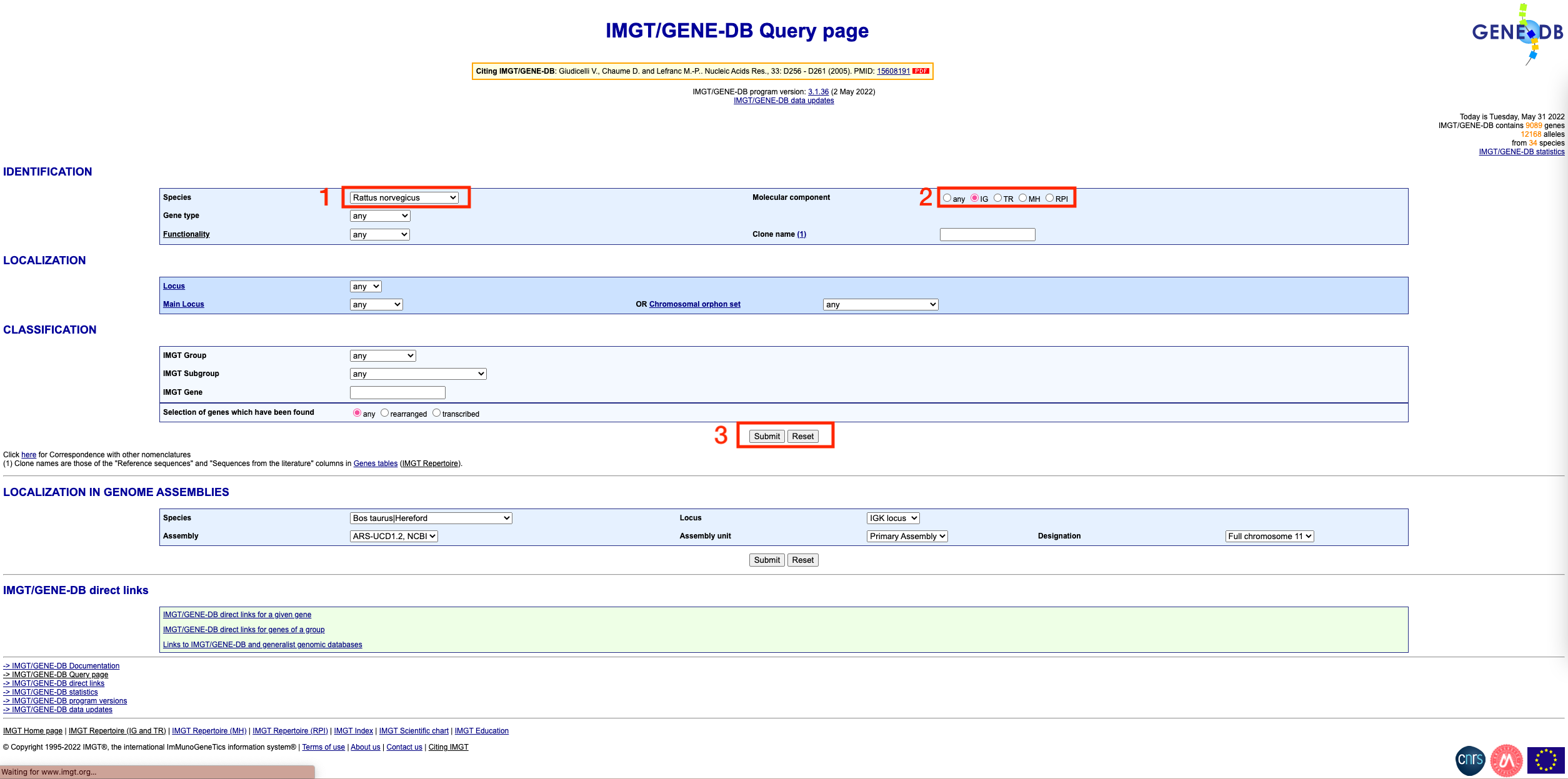
You should see a page that looks like this:
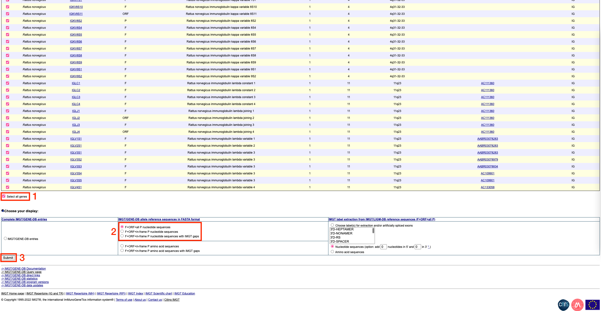
To get the sequences in fasta format, scroll down to the bottom of the page and click on the ‘select all genes’ tickbox. Then, choose ‘F+ORF+all P nucleotide sequences’ under the ‘IMGT/GENE-DB allele reference sequences in FASTA format’ section. Finally, click submit.

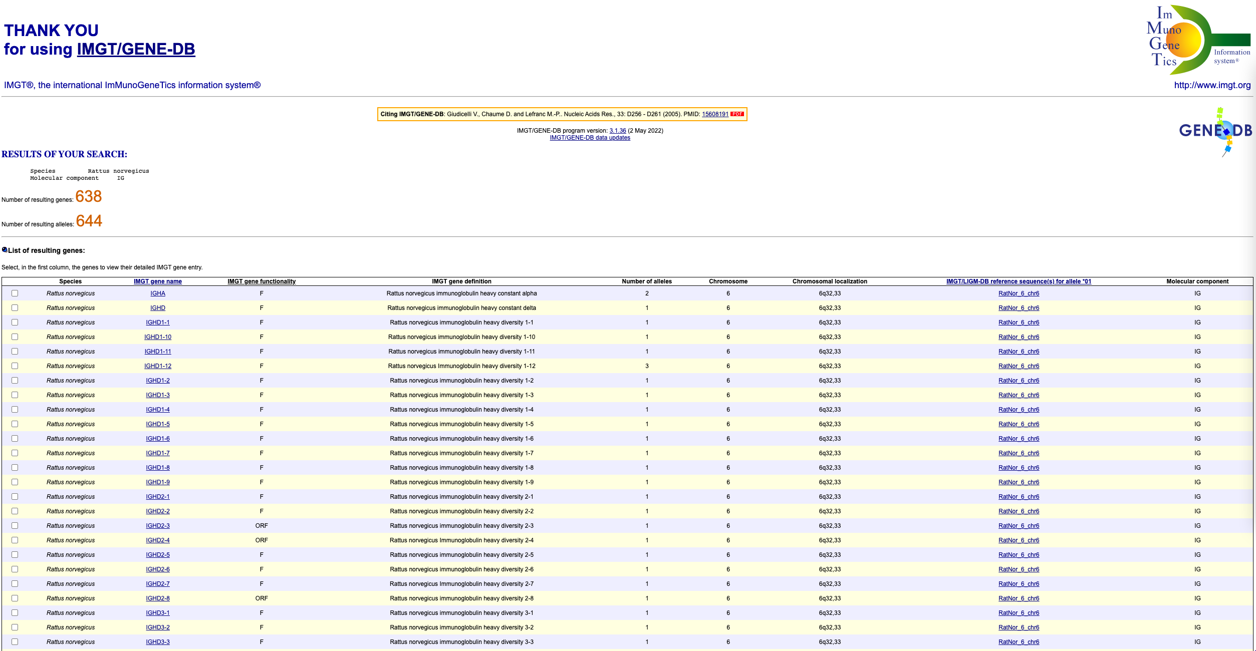
You should see a page that looks like this:
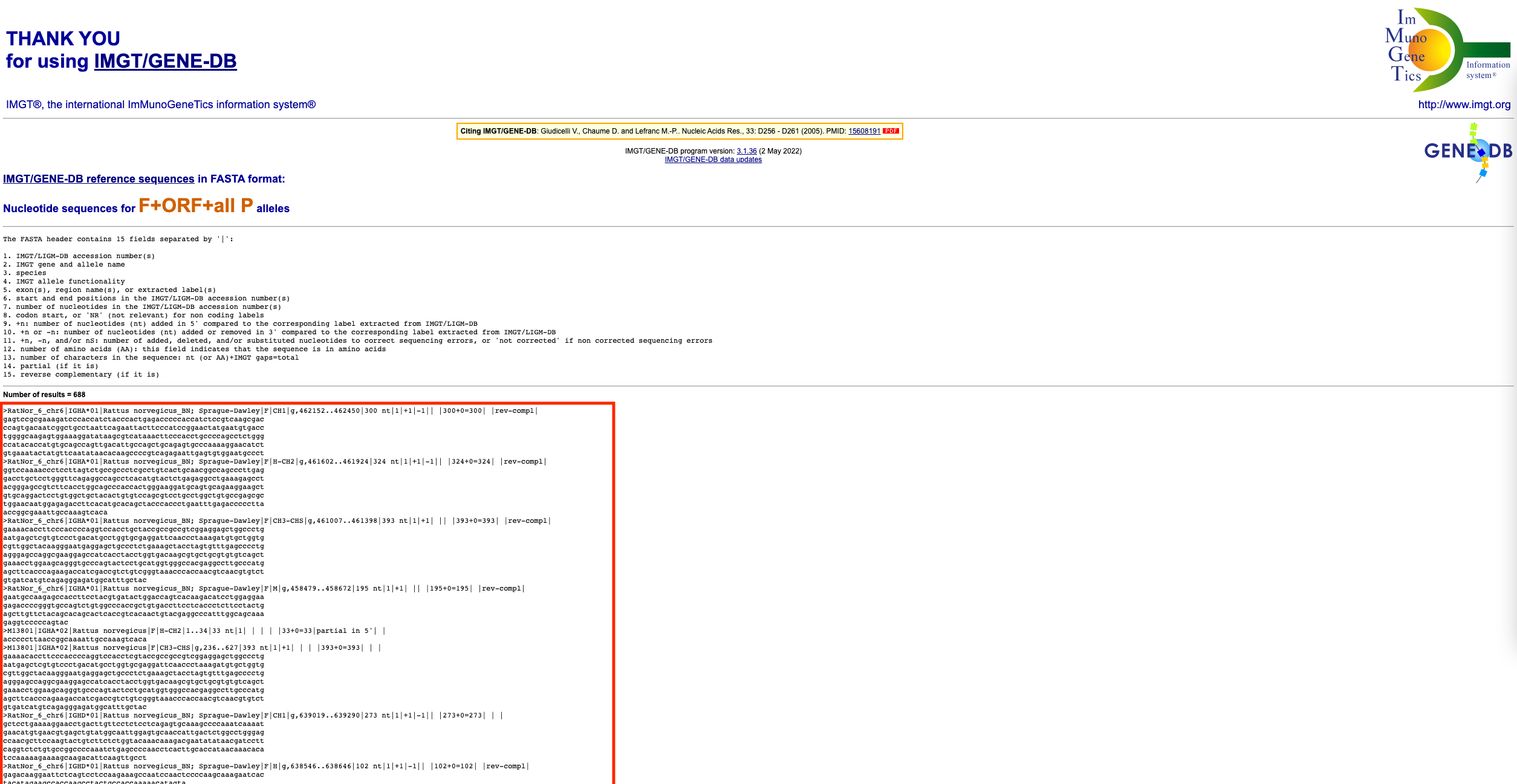
Copy the fasta format sequences (everything below the ‘Number of results’ line, as indicated by the red box above. Paste these sequences into a text editor (e.g. TextEdit on Mac or Notepad on Windows). Save this file with a .fasta extension (e.g. variable_and_constant_references_rattus_norvegicus.fasta)
Done!

The constant region only reference file can be prepared in the same way, except in the second step you should select ‘constant’ from the ‘Gene type’ dropdown box: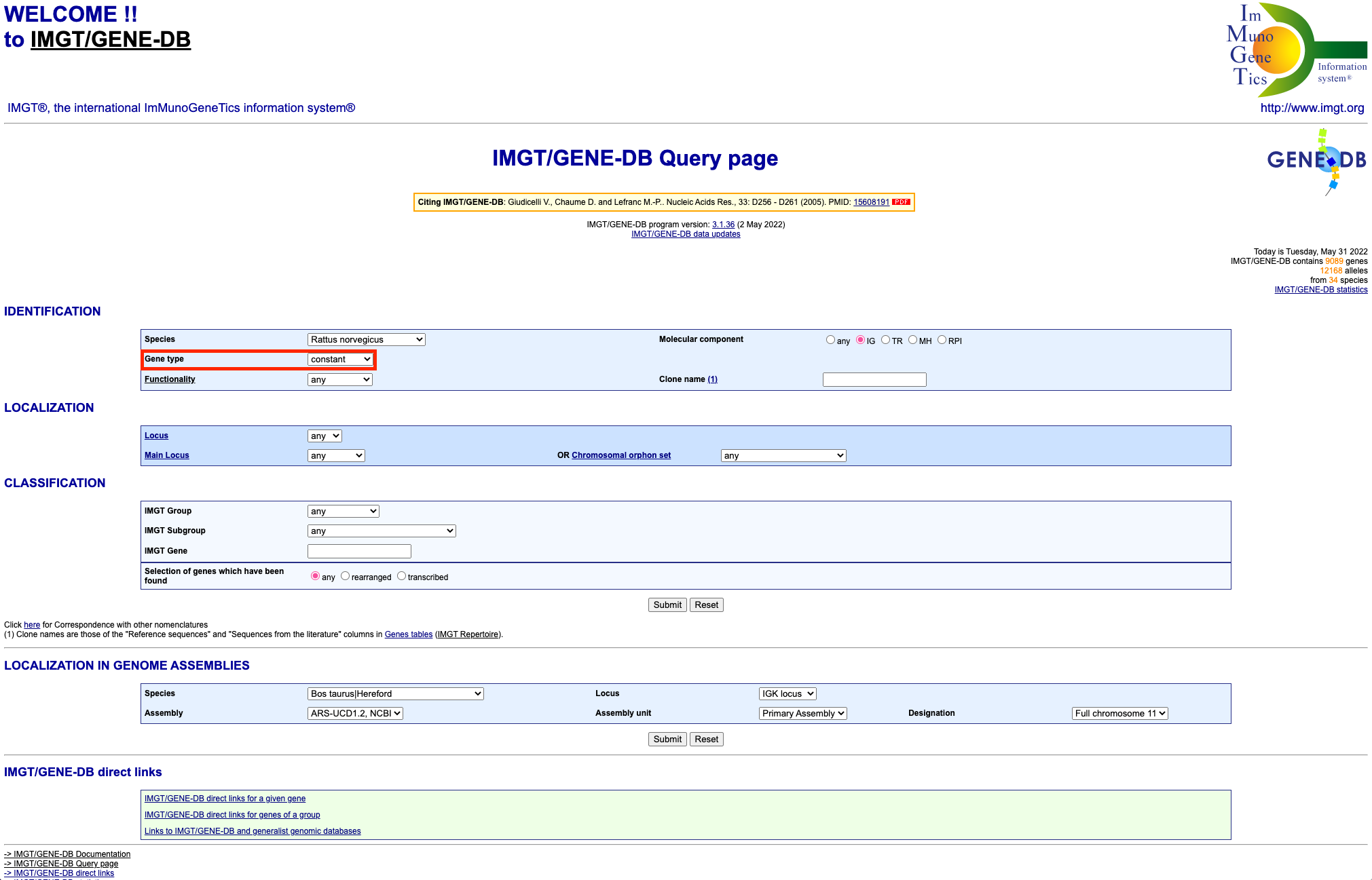

Using the IgBLAST webserver

This section describes how to use the IgBLAST webserver. Note that currently, only human, mouse, rat, rabbit and rhesus monkey are available through this tool (for other organisms, you must use the command line IgBLAST or an alternative tool as described in the read grouping section).

Visit the IgBLAST webpage
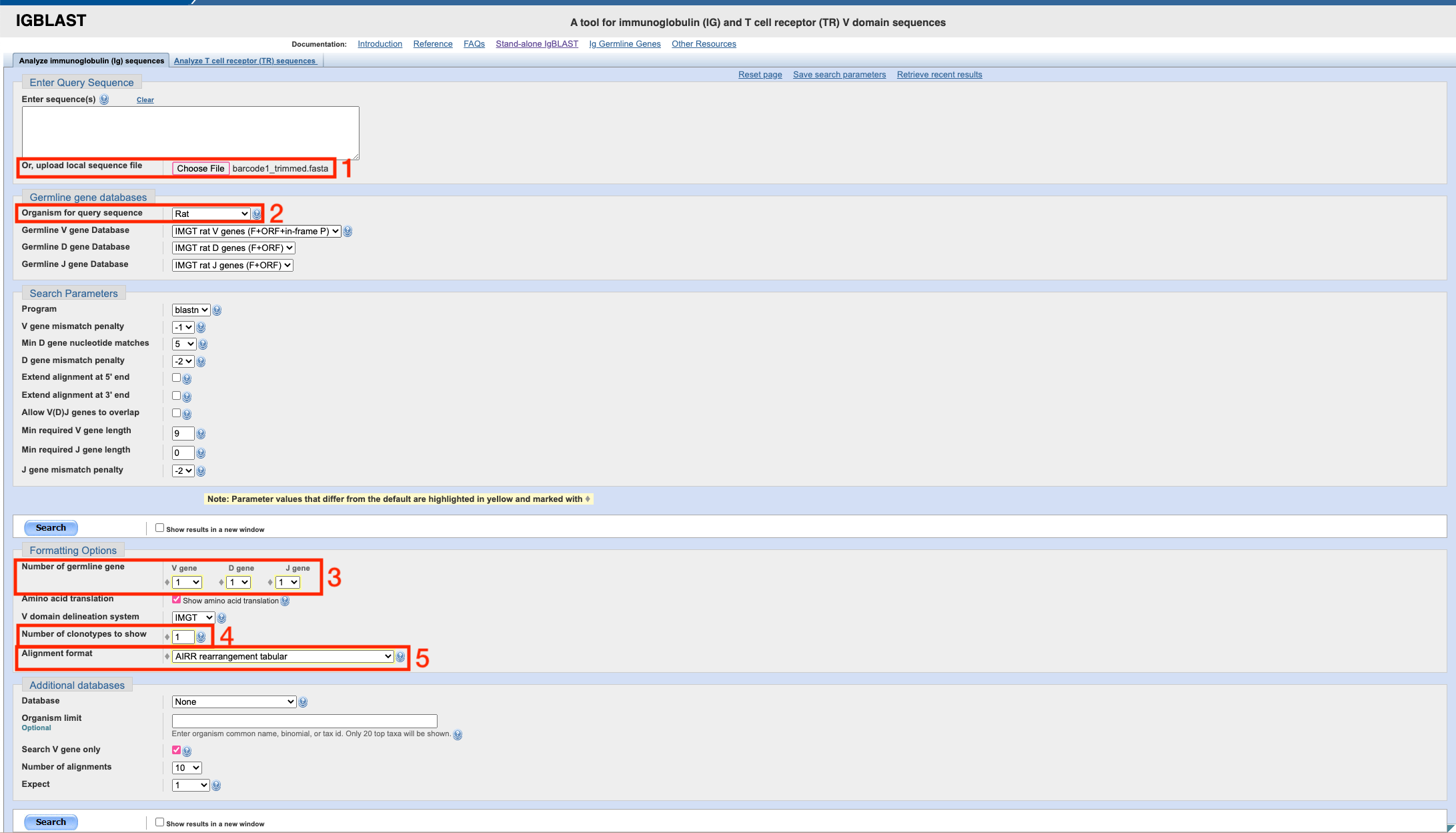
Upload your trimmed .fasta file (see read trimming section) and change the following settings:

After uploading the file, you need to select your organism from the drop down box, and then under formatting options choose ‘1’ for the number of V, D and J genes to display. Set the ‘number of clonotypes to show’ to ‘1’ (this won’t affect results, just a summary table we don’t care about) and the ‘alignment format’ to ‘AIRR rearrangement table’.

Then, press ‘search’ and after a short wait, you should see a page that looks like this:

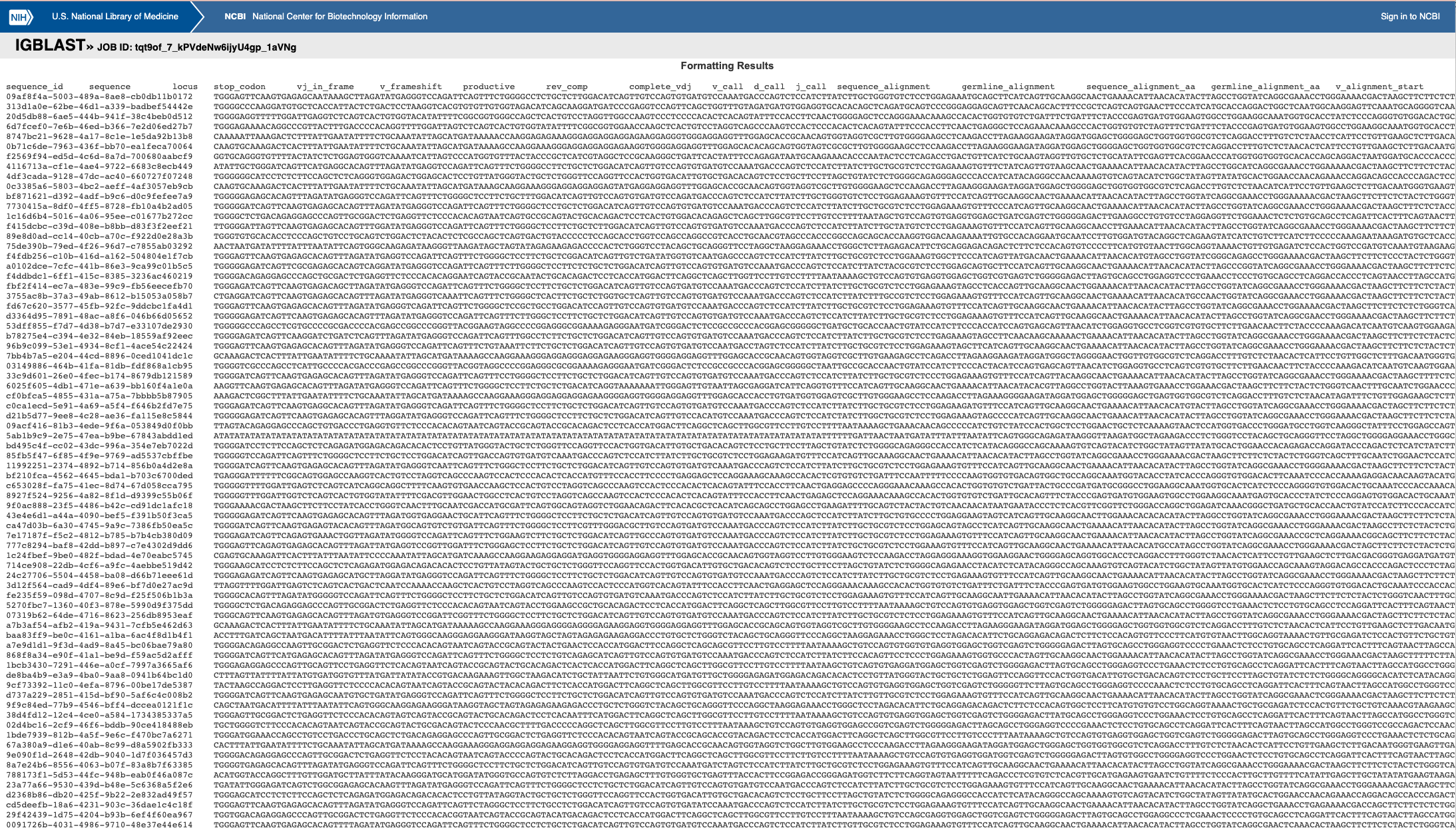
Scroll to the bottom of the page, and select all rows of the first table, as shown in the following image:
Copy paste that first table into a text editor and save it as a .tsv file (for example, library_A_igblast_pre_consensus.tsv). This file can then be used to continue with the read grouping step.

References

Bradbury, Andrew R. M., Nathan D. Trinklein, Holger Thie, Ian C. Wilkinson, Atul K. Tandon, Stephen Anderson, Catherine L. Bladen, et al. 2018. “When Monoclonal Antibodies Are Not Monospecific: Hybridomas Frequently Express Additional Functional Variable Regions.” mAbs 10 (4): 539–46. https://doi.org/10.1080/19420862.2018.1445456.

NAb-seq bioinformatics tutorial (old)

Kathleen Zeglinski

2022-11-15

Introduction

Software required

Input files

Quality control (QC)

QC with NanoComp

Identification of antibody reads

Aligning reads to the antibody reference sequences

Extracting antibody reads

Read trimming

Grouping by germline genes

Annotation of variable regions using IgBLAST

Annotation of constant regions using minimap2

Grouping reads by germline genes in R

Combining the variable and constant calls

Grouping the reads

Preparing for consensus calling

Consensus calling

Final annotation and analysis

Annotation of variable regions using IgBLAST

Annotation of constant regions using minimap2

Further analysis in R

Summary

Appendices

Preparing the reference files from IMGT

Using the IgBLAST webserver

References